Is the simulated market just the model remembering 2019 to 2022?

No. The stylized facts are statistics of daily moves across 100 stocks, such as how often large moves happen and how volatility clusters, which a model cannot recall from what it has read. The path itself differs from the real one: the simulated market rose more in 2019, far less after the COVID crash, and fell more in 2022.

Why use a small open model rather than a frontier model?

Because of what each view needs and how many views there are. A view is read from the model's full probabilities over seven ranges of return, which a model served on our own machine always returns and not every hosted service does. The run also makes 1.21 million calls, which a small model on four GPUs answers for about $130.

How much of the realism comes from the rest of the market?

Some. The rest of the market sets how far a given trade moves a price, using an impact law measured on real markets, which contributes to the fat tails and the short-term reversal. It does not decide when a company's value changes: it revises its valuation only when the agents' views change on fresh information, so when volatility rises and how stocks move together come from the agents.

Agentic Market Simulator, Part 5: Scaling to a Large Number of Agents

This article covers one component of a larger system and makes no claim to replicate a real exchange. Realism will arrive cumulatively across the series: each part is held to its own scope only.

Nothing in this series should be understood as forecasts for prices or investment advice.

Replay of 4-year simulation, from 2019 to the end of 2022: the index and the market map, the 2,000 agents lighting up as they form views, with some agent’s reasoning highlighted.

From a Small Market to a Realistic One

This episode builds on the foundations laid in Episodes 1 to 4: the call auction, the information the agents may see, who acts and when, and how a language model turns what an agent reads into a belief. A market of 20 agents showed that loop working. Here we run it at a more realistic scale: 2,000 agents trading the 100 largest US companies over 1,008 sessions, from 2 January 2019 to 30 December 2022, a period that holds a steady rise, the COVID crash, a boom and a bear market.

The goal here is to produce a realistic market, which should not be confused with replicating historical prices exactly. We compare the simulated prices with the real ones as a reference, and judge the realism of the market on how it behaves.

Setting

Most components are those of the earlier episodes; we list the most relevant parts here:

Universe. The 100 largest US companies by market value at the end of 2018, chosen before the first simulated day.
Information. Each company’s quarterly results on the day they were filed, its news headlines, the macro releases (a dated statistic such as employment, or a central bank decision) and a short daily selection of market-wide press.
Agents. Eight personas of agents: passive indexers, growth investors, risk-averse funds, value quants, retail traders, macro allocators, momentum chasers and panic sellers. Passive indexers simply follow the index and are the only ones who never call the model.
Horizons. Each agent has its own horizon (next month, quarter or year) over which it forms its belief. Note that the same news may mean something different to a short-term trader and a long-term investor.
When agents look. As in Episode 3, an agent reviews a company when its results come out, when there is news about it, when its price moves sharply, or on a routine look at its watchlist.
Beliefs. As in Episode 4, each review is one model call: the model writes a short reason, then gives its probabilities over seven ranges of return, which are transformed into a valuation and a conviction.
Trading. Each view becomes an order in the daily auction of Episode 1. An agent trades toward the position its view implies, and only when it is far enough from it, as investors facing trading costs do (Constantinides 1986).
Short selling and borrowing. Some agents may sell short and some retail accounts may borrow to invest, in the shares observed among US funds and retail investors (Chen, Desai and Krishnamurthy 2013; Kelley and Tetlock 2017), under simplified versions of the US rules.

Running It at Scale

Each simulated session, every review due that day is sent to the model at once. The model used here is Qwen3.5-9B, served by vLLM on a single machine with 4 GPUs. Once the session’s views are in, the 100 auctions clear together. Every review is stored with its reasoning, so the whole run can be replayed and inspected afterwards, as done in the video above.

2,000

agents

100

companies

1,008

trading sessions

1.21 million

model calls

1.89 billion

input tokens

87 million

output tokens

15.8 hours

on one 4-GPU machine

≈ $130

of compute

The model is small and served on a dedicated machine, so a call costs only GPU time, with no price per token, and a session’s reviews are sent together, so the four GPUs stay busy. The simulation for this article ran at about 21 calls a second, and each of the 1.21 million agent decisions cost about a hundredth of a cent.

What the Market Did

Figure 1 shows the simulated index next to the real index of the same companies. This comparison is only a visual check. The simulated market is one of many paths the same market could have taken, so we do not expect it to retrace history, and a very close match would be surprising. We therefore compare the two qualitatively. The simulated market has the broad shape of the four years: a rising 2019 (+38 percent against a real +30), a crash in March 2020, a rising 2021 (+24 against +28) and a bear market in 2022 (−31 against −21). It misses the strength of the 2020 recovery, and ends the four years up 24 percent against 62. Running the simulation again from other starting points, or with other parameters, would produce other paths and surface other patterns.

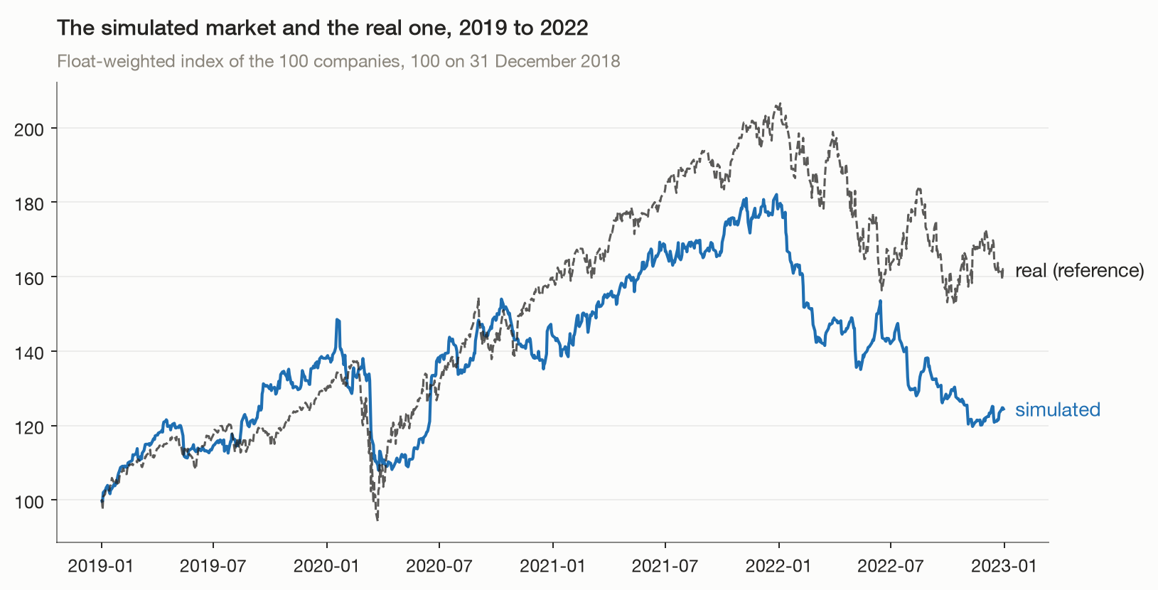
Line chart of two float-weighted indices of the same 100 companies from 2019 to 2022, both starting at 100. The simulated index rises to about 148 by January 2020, falls to about 108 in March 2020, rises to about 180 by the end of 2021 and falls to about 124 by the end of 2022. The real index, dashed, rises to about 138, falls to about 94 in March 2020, rises to about 205 by the end of 2021 and ends 2022 near 162.

Figure 1. The simulated index and the real one, 2019 to 2022. The real index is a reference, not a target.

Figure 2 follows the COVID crash day by day. Note that the simulation does not have complete news coverage: the agents read their companies’ results and headlines, the macro releases and a short selection of market-wide press, which is far less than real investors follow, so their reactions should be expected to differ. The simulated market did not react to the last week of February, when the real one fell 11 percent as outbreaks spread outside China (the simulated one rose 2 percent). It fell once the pandemic was declared: on 11 March both markets lost about 5 percent, and on 12 March the simulated one lost 6 percent against a real 10. Its low came on 24 March, one session after the real low, 27 percent below its January peak, against 32 percent below the February peak for the real market. What it missed most is the rebound: the real market rose 8 percent on 24 March, after the Federal Reserve announced unlimited asset purchases, and 30 percent by the end of April, while the simulated one recovered 2 percent.

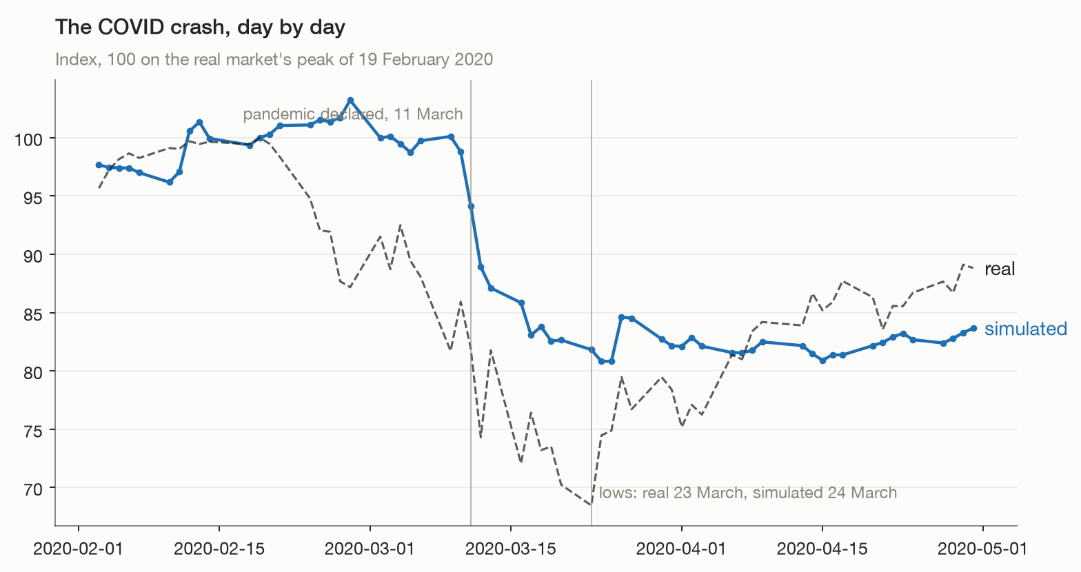
Daily line chart from February to April 2020 of the simulated and real indices, both set to 100 on 19 February 2020. The real index falls steadily from late February to about 68 on 23 March, then recovers to about 89 by the end of April. The simulated index stays near 100 until 10 March, drops to about 82 by 23 March, reaches its low on 24 March and stays between 81 and 84 through April. Vertical lines mark the pandemic declaration on 11 March and the lows of 23 and 24 March.

Figure 2. The COVID crash, simulated and real, with both indices set to 100 on 19 February 2020. The simulated market reacts to the pandemic declaration but neither anticipates it nor rebounds with the real one.

Large moves

In real markets, large daily moves happen far more often than a normal distribution, the bell curve that many financial models assume, would predict. A realistic simulated market should show the same, so this is a useful first check. To make companies comparable, we express each daily return in units of that company’s typical daily move (its standard deviation), then count how often moves of each size occur over the four years, 100,800 company-days in all. Figure 3 compares the simulated market, the real one and the bell curve. We treat it as a sanity check, not a test of ultimate validity in itself.

Under a normal distribution, a move larger than four standard deviations should happen about 6 times in 100,800 company-days. The simulated market had 354 such moves and the real market 767. Large moves in the simulated market are about 55 times more frequent than a normal distribution allows, against about 120 times in the real market: the simulated tails are fat, though not as fat as the real ones.

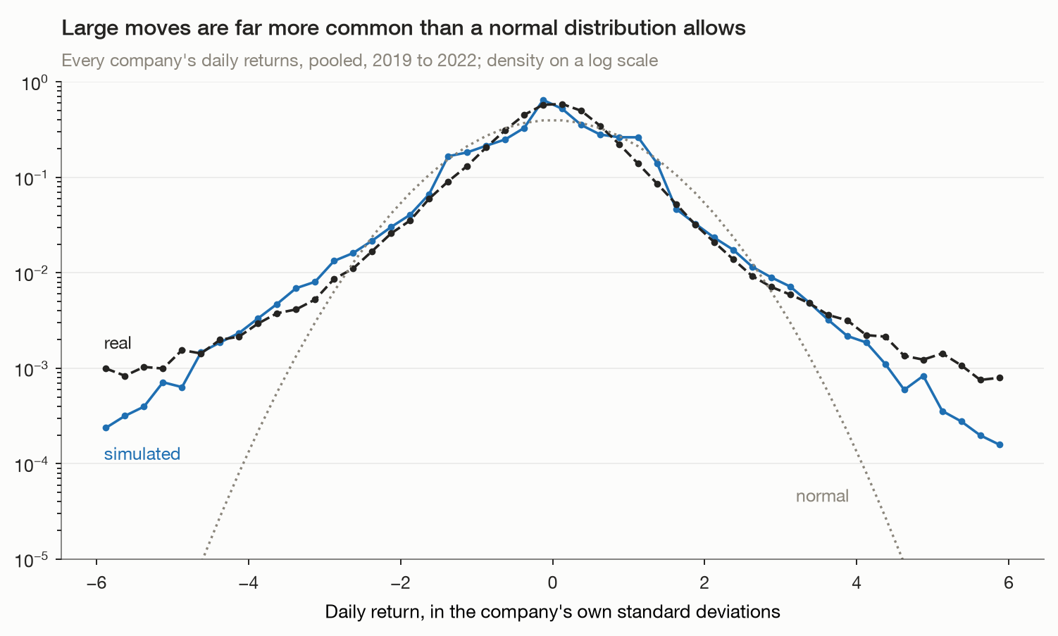
Density on a log scale of every company's daily return in its own standard deviations, 2019 to 2022, for the simulated market, the real market and a normal distribution. The simulated and real densities overlap closely between minus four and plus four standard deviations and both lie far above the normal curve beyond three standard deviations. Beyond five standard deviations the real density stays near one in a thousand while the simulated one falls toward one in five thousand. The normal curve drops below one in a hundred thousand before four and a half standard deviations.

Figure 3. Daily returns of every company, in its own standard deviations, simulated, real and normal. Note the log scale: both markets have far more large moves than the bell curve, the real one more than the simulated one.

Judging Realism

Why stylized facts

Stock prices are very hard to predict, but the way they move is not random in every respect. Across markets, countries, decades and asset classes, daily returns share a set of statistical regularities: large moves happen far more often than a bell curve allows, calm and turbulent periods come in clusters, falls raise future volatility more than rises do, trading volume rises with volatility, and stocks move together more in turbulent times. Cont (2001) collected them under the name of stylized facts.

They became the standard test for market models for a simple reason. The real path of 2019 to 2022 happened once, and does not say anything about what could have happened. The stylized facts hold in most markets and periods, so a model that reproduces them has reproduced how a market produces prices, not one specific history. This is why we judge the simulator on them, and treat the real price path as a qualitative reference only.

Metrics

We measure 19 facts over the four years, covering returns, volatility, volume and how stocks move together. Each has a band from the literature, and a fact passes when the run’s measure falls inside its band. The real prices of the same companies over the same sessions are measured the same way, as a reference, since real markets do not pass every fact in every period either.

Fact (source)	What is measured	Band	Simulated	Real
Returns
No autocorrelation, stocks (Cont 2001)	a stock’s return against the previous day’s	−0.1–0.1	0.03 pass	−0.10
No autocorrelation, index (Cont 2001)	the index’s return against the previous day’s	−0.1–0.1	0.27 fail	−0.22 fail
Heavy tails (Gopikrishnan et al. 1998)	tail index of daily returns (lower is fatter)	2–5	3.36 pass	2.61
Excess kurtosis (Cont 2001)	how much fatter than a bell curve, median stock	≥ 1	2.46 pass	9.65
Gain/loss asymmetry (Cont 2001)	skewness of index returns (large falls outnumber large rises)	≤ 0	−0.60 pass	−0.72
Aggregational Gaussianity (Cont 2001)	daily returns fatter-tailed than monthly ones	≥ 0	0.72 pass	8.75
Volatility
Volatility clustering (Cont 2001)	a large move’s link to the next day’s	0.05–0.4	0.12 pass	0.28
Slow decay of volatility (Ding, Granger and Engle 1993)	the same link, 20 sessions apart	≥ 0.05	0.046 fail	0.117
Leverage effect (Bouchaud, Matacz and Potters 2001)	a fall’s link to the volatility of the next 10 days	≤ 0	−0.03 pass	−0.10
Conditional heavy tails (Cont 2001)	fat tails left once volatility is accounted for	≥ 0.3	2.12 pass	4.28
Volume
Volume moves with volatility (Karpoff 1987)	a stock’s daily volume against the size of its move	≥ 0.1	0.096 fail	0.54
Long memory in volume (Lobato and Velasco 2000)	volume’s link to volume 20 sessions later	≥ 0.1	0.28 pass	0.16
Volume rises on results (Beaver 1968)	volume when results come out, over other days	≥ 1.3	1.26 fail	1.43
How stocks move together
Stocks move together (Plerou et al. 2002)	average correlation between two stocks	0.1–0.6	0.36 pass	0.44
A dominant market mode (Laloux et al. 1999)	share of all co-movement in one common factor	0.15–0.6	0.37 pass	0.46
Correlations rise in turbulent months (Longin and Solnik 2001)	correlation in the most volatile months minus the calmest	≥ 0	0.29 pass	0.41
Diversification (Campbell et al. 2001)	index volatility over a typical stock’s	0.4–0.9	0.64 pass	0.73
The market explains part of each stock (Roll 1988)	share of a stock’s daily moves the index accounts for	0.15–0.6	0.36 pass	0.42
Short-term reversal (Jegadeesh 1990)	a month’s winners against the next month’s	≤ 0.05	−0.05 pass	0.02

Measured over the 1,008 sessions of the run. The real column uses the real prices of the same 100 companies over the same sessions and is a reference: a real value outside its band is marked “fail”. Bands and measures follow the sources named, mostly the facts listed by Cont (2001).

The simulated market passes 15 of the 19 facts; the real prices of the same companies pass 18. For a market built from the ground up, where none of these facts is written into the simulator, this suggests a statistical behavior that is relatively realistic. It is not, however, a perfect match: several measures are weaker than in the real market even where they pass, and the 4 facts that fail concern how quickly the market absorbs market-wide news and how strongly trading responds to large moves and to results, which are part of the limitations of the simulation presented here.

Contrast with Traditional Market Simulations

Two families of models have long been used to simulate markets. Statistical models, such as GARCH (Engle 1982; Bollerslev 1986), describe returns directly. They reproduce volatility clustering because it is written into their equation, and they say nothing about who trades or why, so they cannot answer what would happen under a different rule or a different crowd of investors.

Agent-based models simulate the traders. The Santa Fe Artificial Stock Market (Arthur et al. 1997) and the model of Lux and Marchesi (1999) showed that a few simple trading rules, such as following trends or betting on a return to fundamentals, can produce several stylized facts; Gode and Sunder (1993) showed how much of a market’s behavior comes from its structure even when traders are random. These agents follow a rule with a handful of parameters, usually on one or a few synthetic assets, and the parameters are set so that the facts appear.

Our agents follow no hardcoded trading rule. Each one reads the information a real investor would read about a real company, its own portfolio and its own record, and writes down a judgment, which becomes its view. No specific rule for trend following, herding or panic is written into them, and every decision can be read back in the agent’s own words. The stylized facts above come out of the interaction of these readings in the auction. This is what makes the simulator useful for “what if” questions: change a rule of the market, or the news, and observe how the agents respond.

Markets of language-model agents are a recent line of work, and most of them are small: a few to a few hundred agents, one to a dozen assets, and days to months of trading. TwinMarket (Yang et al. 2025) runs up to 1,000 language-model agents on ten industry indices over a few months and reports four stylized facts. MarketSim (Piao et al. 2026) grounds its market in real news and real stocks and simulates more than 15,000 participants, most of them rule-based, over scenarios of a few days, and tests five stylized facts. To our knowledge, no published simulation combines more than a thousand agents that consult a language model for every decision, a universe of about a hundred real companies, several years of daily trading, and a panel of stylized facts of this size.

Limitations

The simulator presented in this series is a deliberately simplified version: its purpose is to share the building blocks of a powerful and realistic market simulator. Several limitations are addressed in the more capable versions we use internally. The main limitations of this experiment are:

Crashes are too slow and too shallow. The simulated market absorbs market-wide news over several sessions, where the real one reacted at once and then rebounded, as the COVID crash shows. One reason is coverage: the agents read a selection of results, headlines and macro releases, not the full flow of news that real investors follow.
Volume reacts too little to large moves and to results.
Agents see less than real investors. They read filings, a selection of news and prices, but not analyst estimates, earnings calls, order books, option markets or the prices of other assets, all of which real investors watch.
A sample of the market. The universe is 100 large US companies, and the 2,000 agents are far fewer than the investors in a real market.
Personas. The personas should be more diversified and calibrated against how real investors trade.

A market that behaves realistically can be used as a laboratory. In the next episode of this series, we will present a realistic use case for such a framework. We will take this run back to February 2020 and replay the COVID crash under a ban on short selling, as six European countries imposed in March 2020, to see what the ban changes and how that compares with what the real bans did.

Work with us

Would you like a production or business version of this simulator: on your own universe of assets, with your own data or models, or to explore your own scenarios? We would be glad to discuss it.

References

Cont, “Empirical properties of asset returns: stylized facts and statistical issues”, Quantitative Finance (2001): the list of stylized facts, and most of the measures and bands of the test.
Gopikrishnan, Meyer, Amaral & Stanley, “Inverse cubic law for the distribution of stock price variations”, European Physical Journal B (1998): the tail index of stock returns, about 3.
Ding, Granger & Engle, “A long memory property of stock market returns and a new model”, Journal of Empirical Finance (1993): the slow decay of the autocorrelation of absolute returns.
Bouchaud, Matacz & Potters, “Leverage effect in financial markets: the retarded volatility model”, Physical Review Letters (2001): the leverage effect in stock returns.
Karpoff, “The relation between price changes and trading volume: a survey”, Journal of Financial and Quantitative Analysis (1987): volume rising with the size of price moves.
Lobato & Velasco, “Long memory in stock-market trading volume”, Journal of Business & Economic Statistics (2000): the persistence of trading volume.
Beaver, “The information content of annual earnings announcements”, Journal of Accounting Research (1968): trading volume rising when results are announced.
Laloux, Cizeau, Bouchaud & Potters, “Noise dressing of financial correlation matrices”, Physical Review Letters (1999): the dominant market mode in stock correlations.
Plerou, Gopikrishnan, Rosenow, Amaral, Guhr & Stanley, “Random matrix approach to cross correlations in financial data”, Physical Review E (2002): the average correlation of stocks and the market mode.
Longin & Solnik, “Extreme correlation of international equity markets”, Journal of Finance (2001): correlations rising in turbulent markets.
Campbell, Lettau, Malkiel & Xu, “Have individual stocks become more volatile? An empirical exploration of idiosyncratic risk”, Journal of Finance (2001): index volatility against stock volatility, the diversification measure.
Roll, “R²”, Journal of Finance (1988): the share of a stock’s moves explained by the market.
Jegadeesh, “Evidence of predictable behavior of security returns”, Journal of Finance (1990): the short-term reversal of monthly returns.
Constantinides, “Capital market equilibrium with transaction costs”, Journal of Political Economy (1986): trading only when far enough from the target position.
Chen, Desai & Krishnamurthy, “A first look at mutual funds that use short sales”, Journal of Financial and Quantitative Analysis (2013): the share of US equity funds that sell short.
Kelley & Tetlock, “Retail short selling and stock prices”, Review of Financial Studies (2017): retail short selling.
Engle, “Autoregressive conditional heteroscedasticity with estimates of the variance of United Kingdom inflation”, Econometrica (1982), and Bollerslev, “Generalized autoregressive conditional heteroskedasticity”, Journal of Econometrics (1986): statistical models of volatility clustering.
Arthur, Holland, LeBaron, Palmer & Tayler, “Asset pricing under endogenous expectations in an artificial stock market”, in The Economy as an Evolving Complex System II (1997): the Santa Fe Artificial Stock Market.
Lux & Marchesi, “Scaling and criticality in a stochastic multi-agent model of a financial market”, Nature (1999): stylized facts from simple trading rules.
Gode & Sunder, “Allocative efficiency of markets with zero-intelligence traders”, Journal of Political Economy (1993): how much of a market’s behavior comes from its structure.
Yang et al., “TwinMarket: A scalable behavioral and social simulation for financial markets”, NeurIPS (2025): a market of language-model agents, for comparison.
Piao, Liu, Huang, Huang, Li, Wang & Li, “MarketSim: Simulating stock markets with large-scale generative agents”, ICML (2026): a market of real stocks and real news with language-model and rule-based participants, for comparison.

Agentic Market Simulator Part 5: Scaling to a Large Number of Agents

Agentic Market Simulator · Part 5 of 6

TL;DR