
Agentic Market Simulator Part 1: Engine and Environment
Agentic Market Simulator · Part 1 of 9
This series builds a discrete-time stock market simulator in which the participants are AI agents represented by small language models. Across nine episodes of this series we cover the auction system, the information the agents are allowed to see, how they make decisions, what bias is present in language model weights, the agent personas and their memory, the cost of running a large population, and what the finished thing is useful for in practice. It should be understood as a research simulator, not a live trading system.
- ▸ 1Engine and Environmentyou are here
- 2Universe, Information and Leakage
- 3Personas, Memory and Track Record
- 4Scaling to a Large Number of Agents
- 5Validation and Calibration
- 6Market Regimes and Persona Proportions
- 7Impact, Capacity and Backtesting
- 8Visualization
- 9Putting it Together
TL;DR
This article is the first episode of this series. It introduces the topic, sets the scope and builds the market auction system. We use one synthetic asset, one clearing event per simulated day, and agents that hold cash and shares and act under budget constraints. There is no language model involved in this first episode. We are only introducing simplified trading agents which possess rudimentary capabilities like following budget constraints and bidding according to a private signal. We note that the simple mechanisms we use here are enough to enable the agents to track the underlying asset’s fundamental value within one percent and produce realistic behavior.
This article covers one component of a larger system and makes no claim to replicate a real exchange. Realism will arrive cumulatively across the series: each part is held to its own scope only.
Nothing in this series should be understood as forecasts for prices or investment advice.
Introduction to the Series
The goal of the series is to show how to design a simulator where a population of language-model agents trades against each other over a multi-year horizon, so that, for example, we can ask counterfactual questions like what happens if the market is mostly momentum traders, how much alpha a strategy keeps once the other participants react to it, who is paying for a strategy's gains, or how exogenous political events impact a strategy's performance.
Each episode of the series will cover one component of the system, and each component should be realistic enough in its own domain, not expected to produce a realistic market by itself. For example, the auction system is responsible for translating orders into a price, deciding who gets filled, and defining what an account is allowed to do. It is not responsible for whether traders panic, herd, change their minds, or read the news. In each episode, we will measure realism within a restricted perimeter and highlight what the integration with the next component will bring.
In this first episode, we design the auction mechanism which determines the price of each asset based on supply and demand. We focus on a single synthetic asset, 250 trading days, 400 simplified agents, and rule-based behaviour to validate the design of this component.
Trading Frequency
In real equity markets, orders arrive microseconds apart, they queue, and positions in that queue matter. In this series, we will focus on one step per trading day, which makes the problem tractable and allows us to focus on high-level modelling decisions. By doing so, we lose intraday latency arbitrage, queue priority, and anything that depends on the order in which two participants act within a day. However, we preserve the feedback loop between what agents believe, what they trade, and what the price does in response, which is what we are interested in modeling here.
The daily frequency affects the definition of “the order book”: with one clearing event per day there is no continuous matching and no bid-ask spread in the usual sense. What we have is a call auction: everyone submits limit orders, they are crossed once, and every trade that day happens at the same price.
Price Computation
Aggregate demand is the total quantity of buy orders willing to pay at least , and aggregate supply is the total quantity of sell orders willing to accept at most . One is decreasing in price, the other increasing. The clearing price is the one that lets the most shares change hands:
We break ties with a commonly used rule: first prefer the price with the smaller imbalance , then the price closest to the previous close. Only prices that someone actually quoted can win, so the search is over a finite set.
The naive implementation checks every candidate price against every order: for each of up to distinct prices it resums quantities across all orders, which gives a complexity of . That is 900 million for 30,000 orders. Sorting each side by price once and precomputing cumulative demand and supply turns every per-price lookup into a binary search instead of a fresh sum, bringing the total cost down to :
candidates = np.unique(np.array([o.price for o in orders]))

# demand(p) = quantity of buys priced at or above p
buy_suffix = np.concatenate([np.cumsum(buy_q[::-1])[::-1], [0]])
demand = buy_suffix[np.searchsorted(buy_p, candidates - PRICE_EPS, side="left")]

# supply(p) = quantity of sells priced at or below p
sell_prefix = np.concatenate([[0], np.cumsum(sell_q)])
supply = sell_prefix[np.searchsorted(sell_p, candidates + PRICE_EPS, side="right")]

volumes = np.minimum(demand, supply)
best_volume = int(volumes.max())

# Maximum volume first, then the smaller imbalance, then the price
# closest to the previous close.
tied = np.flatnonzero(volumes == best_volume)
imbalance = np.abs(demand[tied] - supply[tied])
tied = tied[imbalance == imbalance.min()]
pick = tied[np.argmin(np.abs(candidates[tied] - reference_price))]
Orders strictly better than the clearing price are entitled to a full fill. Orders sitting exactly at it share whatever volume is left, pro rata, with a largest-remainder rule so that no share goes missing to rounding. If the book does not cross at all, there is no trade and the previous close carries forward. In our runs, we saw that some percentage of sessions failed to trade, which would not happen to a real large cap. In reality, there are dedicated liquidity providers that quote continuously on both sides, and this engine has none. Another simplification in this episode is that every order is a limit order and the auction is single-pass, with no indicative price for agents to react to. In later episodes, we will add market orders, and a call phase that lets agents revise their orders.
We also set a daily price limit of ±20 percent, log-symmetric around the previous close. It is applied per order as the agents generate them, so any level priced outside the band is dropped before the auction runs. The clearing price is therefore bounded by construction. Note that a linear version, last_price × (1 ± 0.20), would clip the sell side harder than the buy side and leave a persistent order-flow imbalance.
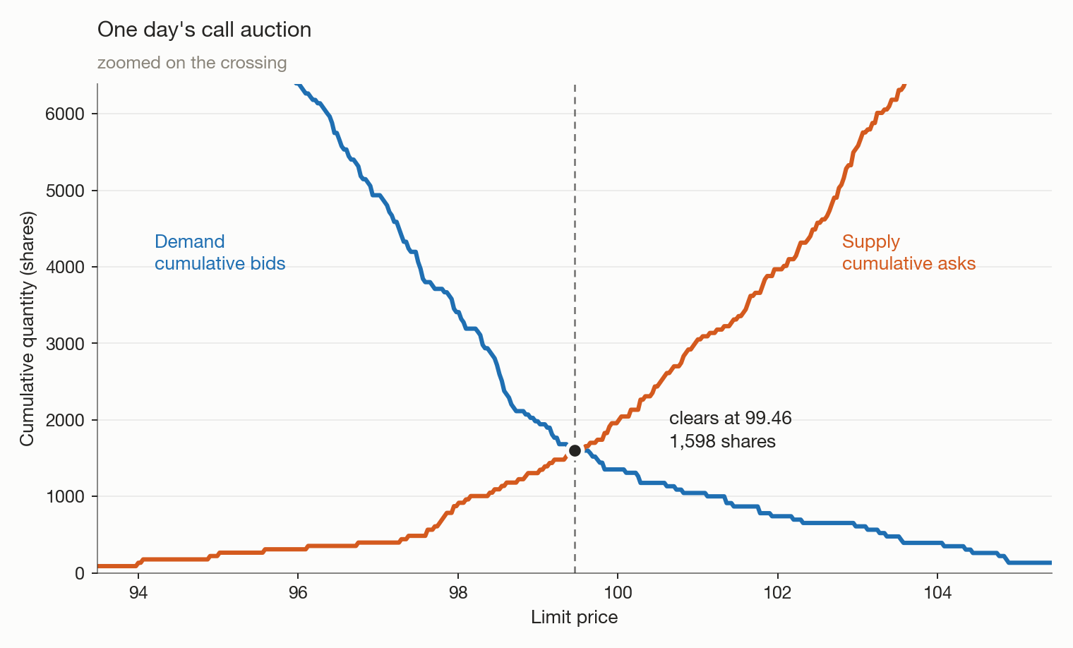
One day’s auction, zoomed on the crossing. Both curves run to tens of thousands of shares at the edges of the daily price limit, so the full range hides the only part that matters.
Agents' Actions
In this section, we introduce a set of simple, hand-coded agent behaviors whose only job is to generate order flow realistic enough to exercise the auction, so that we can check that the mechanism itself does not have obvious flaws before developing any real intelligence. In later episodes, we will expand on the agent capabilities that we describe here, although none of the current assumptions restrict how language-model agents will operate:
- Private signal and persistence, an AR(1) process with a hardcoded persistence, stands in for a model reading financials, prices and news. The actual model will be introduced in Part 3 of this series.
- A logistic target-position rule stands in for persona-specific risk appetite, which will also be introduced in Part 3.
- The fundamental value itself is a synthetic random walk, standing in for real market data, which will be introduced in Part 2.
Naive agents let us verify that the mechanism works before any language model comes into play. Understanding how to design naive agents which produce realistic market behavior is a stepping stone toward designing more complex language-model agents.
Modeling the fundamental value and private signals
We assume the single asset we are considering has a latent fundamental value that follows a discrete-time geometric random walk. No agent observes it. Each agent sees a private, noisy version of it, and the disagreement between those private signals is the only reason anyone trades. Note that this modeling is used only for this episode, and will be replaced by real market data in later episodes.
- : the true fundamental value on day , unobserved by agents.
- : the fundamental’s volatility.
- : a standard normal shock for day .
- : agent ’s private signal on day .
- : agent ’s signal noise on day .
- : the dispersion of that noise across agents.
How long an agent keeps its view strongly influences its willingness to trade every day, and therefore turnover. A naive version could redraw independently every day: each agent therefore re-derives its entire thesis every morning, which is quite unrealistic. We ran this as an experiment. The results showed that agents’ valuation moved about 7 percent a day when the fundamental had moved 1.2 percent, and the market turned over 4.5 percent of its shares daily against the 0.5 to 1 percent a real large cap does. This is a simple example of unrealistic market behavior caused by a modelling shortcut.
We will model the signal error as an AR(1) process, scaled so that the cross-sectional dispersion stays at whatever the persistence is.
def advance_signal(eta, cfg, rng):
    """Move each agent's private view one day forward.

    The scaling on the innovation keeps the stationary variance at
    sigma_signal^2 for any persistence, so dispersion and persistence
    stay independent dials.
    """
    rho = cfg.signal_persistence
    shock = rng.normal(0.0, 1.0, len(eta))
    return rho * eta + math.sqrt(max(0.0, 1.0 - rho ** 2)) * cfg.sigma_signal * shock
We are not fitting to a turnover target. Instead, we take it from the cadence of the information agents will eventually read: company financials which arrive quarterly, so a view derived from them should be revised on roughly that schedule. gives a half-life of 69 trading days, and in our simulations this yields daily turnover of 0.12 percent. This is below the 0.5 to 1 percent a real large cap turns over, but turnover is set by how long beliefs persist, which is currently a placeholder. Note that the agent’s valuation still moves every day, because it tracks the fundamental.
From Signal to Demand Curve
The important design decision is what an agent does with that signal. The obvious choice, comparing the signal to yesterday’s close and buying if it looks cheap, would not work. Every agent flips side in unison as soon as the price crosses the fundamental, the price overshoots, and everyone flips back the next day. We measured a lag-1 return autocorrelation of about , which is nothing like a real daily series. Partial participation does not fix it either, because the agents who do act still all act the same way.
What fixes it is letting the agents submit their entire demand function as a function of the price. Then the auction system allocates accordingly. This is a standard way to model auctions. Here, we will use the following functional form, also inspired by the literature, which makes sure the quantity is bounded by a fixed value.
- is the number of shares the agent wants to hold for a price .
- is the price being considered, the same price used to build the demand schedule below.
- is the agent’s private valuation, taken from the signal equation above.
- is the position limit, the largest number of shares the agent is allowed to hold.
- is the demand sensitivity. A larger value makes the target move more sharply as the price moves away from the agent’s valuation.
In practice, an agent submits its whole demand curve, sampled on a grid of price levels, and each level becomes one limit order. The schedule is cumulative, so the orders carry the difference between adjacent levels and filling several at once cannot overshoot the target:
def target_position(valuation, last_price, cfg):
    gap = math.log(valuation / last_price)
    return cfg.max_position / (1.0 + math.exp(-cfg.demand_sensitivity * gap))


def demand_schedule(agent, valuation, last_price, cfg):
    """The agent's whole demand curve, as (price, cumulative shares) rungs."""
    rungs = []
    for i in range(SCHEDULE_RUNGS):
        frac = 2.0 * i / (SCHEDULE_RUNGS - 1) - 1.0          # -1 .. +1
        price = round_to_tick(valuation * math.exp(SCHEDULE_WIDTH * frac))
        delta = target_position(valuation, price, cfg) - agent.shares
        rungs.append((price, int(round(delta))))
    return rungs
Note that the grid is anchored on the agent’s own valuation, not on the last close. If we anchored it on the close, which would give every agent in the market the same nine price levels, the clearing price could only ever land on one of them. Daily returns would come out quantised to almost exactly the quoted margin, and the volatility we would measure would only be artifact of the grid, not a market property. This is the same discreteness bias Gottlieb and Kalay (1985) documented for real markets trading on a fixed tick size, here produced by the agent’s price-level count rather than the exchange’s. Valuations are continuous, so anchoring on them keeps the aggregate curves continuous too.
Budget Constraint
Since agents are submitting demand curves, i.e., several buy orders at different prices before knowing what the price will actually be, the budget constraint is checked against the worst price each order could fill at.
def enforce_budget(agent, orders, cfg):
    """Trim orders until no clearing price can overdraw the agent."""
    kept = []

    cumulative = 0
    for o in sorted((o for o in orders if o.side == BUY), key=lambda o: -o.price):
        by_cash = int(agent.cash // max(o.price, PRICE_FLOOR))
        room = min(by_cash, cfg.max_position - agent.shares) - cumulative
        quantity = max(0, min(o.quantity, room))
        if quantity > 0:
            o.quantity = quantity
            cumulative += quantity
            kept.append(o)

    cumulative = 0
    for o in sorted((o for o in orders if o.side == SELL), key=lambda o: o.price):
        room = agent.shares - cumulative
        quantity = max(0, min(o.quantity, room))
        if quantity > 0:
            o.quantity = quantity
            cumulative += quantity
            kept.append(o)

    return kept
With short selling and leverage switched off, cash and holdings can never go negative, so bankruptcy is impossible by construction. This assumption has to be revisited the moment leverage is considered.
Naive Benchmark: Zero Intelligence Control
Now that we have designed agents that follow a simple, structured rule, it is useful to consider a benchmark that contains no intelligence at all. Running a comparison helps us to understand how much of the final behavior we observe in the market is due to the structure we impose versus the pricing rules used by agents. This will also be useful to understand the incremental value brought by intelligent agents in later episodes. We use Gode and Sunder’s 1993 experiment, which replaced human traders with agents that submit random prices and found that market efficiency barely changed. Their conclusion was that a large part of what looks like trader skill is actually produced by the market mechanism and the budget constraint.
We run three regimes over the identical fundamental path, with identical signals and identical demand schedules. The only thing that differs between regimes is how each price level is set:
def _price_for(regime, side, reservation, last_price, cfg, rng):
    """Price one rung. This function is the whole difference between regimes.

    `reservation` is the marginal value of the increment: the price at which
    this agent is exactly indifferent about holding one more share.
    """
    if regime == "value":
        # Quote at the reservation price, keeping a fixed margin for itself.
        m = cfg.value_margin
        return round_to_tick(reservation * (1 - m) if side == BUY else reservation * (1 + m))

    if regime == "zi-c":
        # Random, but a buyer never bids above its own marginal value and a
        # seller never asks below it. Gode and Sunder's budget constraint.
        draw = rng.random() * cfg.zi_spread
        return round_to_tick(reservation * (1 - draw) if side == BUY
                             else reservation * (1 + draw))

    if regime == "zi-u":
        # Ignores its own valuation completely: a uniform draw around the last
        # close, which can and does land on the wrong side of its own value.
        band = cfg.zi_band * (2.0 * rng.random() - 1.0)
        return round_to_tick(last_price * (1.0 + band))

    raise ValueError(f"unknown regime {regime!r}")
We look at the following metrics to assess the realism of each regime:
- Tracking error is the root mean square gap between the clearing price and the fundamental in logs, . Lower is better.
- Daily turnover is the share of outstanding shares that change hands each day, checked against the 0.5 to 1 percent a real large cap turns over.
- Lag-1 autocorrelation is whether tomorrow’s return can be predicted from today’s. It should be close to zero.
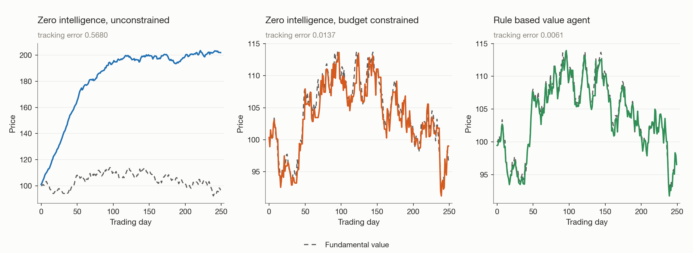
The same fundamental path (dashed) traded by three regimes. Note the differing y-axes: the unconstrained regime reaches roughly twice the fundamental and would flatten the other two panels on a shared scale.
Averaged over eight seeds of 250 days, with the spread across seeds shown for the tracking error:
| Regime | Tracking error | Daily turnover | Lag-1 autocorr. |
|---|---|---|---|
| Zero intelligence, unconstrained | 0.668 ± 0.117 | 32.9% | +0.49 |
| Zero intelligence, budget constrained | 0.0118 ± 0.0008 | 0.06% | −0.19 |
| Rule based value agent | 0.0043 ± 0.0008 | 0.12% | −0.03 |
The first interesting thing to notice is that the constraint does most of the work, as noted in the literature. An agent that picks its price uniformly at random, and is only stopped from bidding above its own valuation, tracks the fundamental to within about 1.2 percent. It has no strategy, no memory and no view. The mechanism plus the budget constraint is doing the price discovery.
The second is that pricing skill still matters: quoting at your own reservation price instead of pricing randomly improves tracking by a factor of under three.
The third is what happens when the constraint is removed. The unconstrained regime cannot be considered a realistic market. The price loses its anchor and drifts to roughly twice the fundamental.
Fixed & Temporary Components
In this first episode, we have introduced the auction system that will be used in our simulated market and used it with simplified agents. The trading agents we have presented are simplified but still follow some structure. The next episodes will build on top of that structure to add intelligence in some areas while preserving some structural design. We summarize in the table below what aspects of the system will be kept and those that will be replaced by real data or more intelligent mechanisms.
| Component | Status | Replaced by |
|---|---|---|
| Clearing rule, allocation, price limits | Permanent | None |
| Accounting, budget constraint, invariants | Permanent | None |
| Event log, seeding, manifest, self-tests | Permanent | None |
| Demand schedule construction | Permanent | Kept, but fed by an agent’s valuation. |
| Private signal and its persistence | Placeholder | Part 3: a model reading financials, prices and news. |
| Logistic target position | Placeholder | Part 3: persona-specific risk appetite. |
| The three regimes | Placeholder | Part 3: personas. |
| Synthetic fundamental | Placeholder | Part 2: real data. |
Replicability
Replicability will be a crucial aspect of this system. Here are some of the important features to implement from the start.
- One config object. Every number the simulation depends on is defined in a single dataclass, and the run manifest is that dataclass serialised next to the results.
- Seeds. Random processes should be properly seeded.
- One event log. We will use an append-only Parquet log with a stable schema.
The code snippets in this article are provided to illustrate some important parts of the code. The complete simulator, including the plotting and the run harness, will be open-sourced on GitHub at the end of the series.
Common questions
Why a call auction and not a real limit order book?
With one clearing event per day, there’s nothing for a continuous double auction to be continuous about. Queue priority and intraday matching only matter if participants can act at different moments within the same step, and ours can’t.
If zero-intelligence agents already track the fundamental, why use language models at all?
Because price discovery isn’t the interesting part. Random agents get a reasonable price but a terrible allocation, and they can’t hold a view, remember being wrong, change strategy after a loss, or react to news. You also can't audit the system to understand market behavior. It's also a baseline that sets the floor for a language-model agent.
References
- Gode & Sunder, “Allocative Efficiency of Markets with Zero-Intelligence Traders”, Journal of Political Economy (1993): the source of the zero-intelligence control.
- Arthur, Holland, LeBaron, Palmer & Tayler, “Asset Pricing Under Endogenous Expectations in an Artificial Stock Market” (1997): the Santa Fe model, the reference point for agent-based markets with heterogeneous beliefs.
- Chiarella & Iori, “A Simulation Analysis of the Microstructure of Double Auction Markets” (2002): demand schedules and inventory effects in an order-driven market.
- Gottlieb & Kalay, “Implications of the Discreteness of Observed Stock Prices”, Journal of Finance (1985): how quantizing prices onto a discrete grid biases measured variance, the effect the close-anchored grid above would have reproduced.