
Agentic Market Simulator Part 3: Attention, or Who Acts and Why
Agentic Market Simulator · Part 3 of 10
This series builds a discrete-time stock market simulator in which the participants are AI agents represented by small language models. Across ten episodes of this series we cover the auction system, the information the agents are allowed to see, how they make decisions, what bias is present in language model weights, the agent personas and their memory, the cost of running a large population, and what the finished thing is useful for in practice. It should be understood as a research simulator, not a live trading system.
- 1Engine and Environment
- 2Universe, Information and Leakage
- ▸ 3Attention: Who Acts, and Whyyou are here
- 4Beliefs, Personas and Track Record
- 5Scaling to a Large Number of Agents
- 6Validation and Calibration
- 7Market Regimes and Persona Proportions
- 8Impact, Capacity and Backtesting
- 9Visualization
- 10Putting it Together
TL;DR
Before an agent can decide what to think, something must determine whether the agent is paying attention at all. This episode separates that question into its own layer, builds it, and calibrates it on its own. We show how this creates a schedule of who acts on which day and for which reason. We can measure and sanity check before moving on to the next phase of letting agents produce beliefs about assets. We note that the process we introduce here produces the activity clustering pattern that Episode 1 could not generate.
This article covers one component of a larger system and makes no claim to replicate a real exchange. Realism will arrive cumulatively across the series: each part is held to its own scope only.
Nothing in this series should be understood as forecasts for prices or investment advice.
Why Trade?
Given the current rapid advances in LLMs, it is very tempting to think that simulating a financial market with AI agents can be done directly by spawning a large number of agents, prompting them to buy and sell, execute, and observe the results. That approach produces something that runs almost immediately, but does not produce anything that looks like a real financial market. This is because it misses the fundamental question that must be answered first:
Why does anyone trade at all?
Milgrom and Stokey (1982) showed that if all participants are rational, share common prior beliefs, and never trade out of force, then no trade happens. This is because there is no disagreement, every actor believes the same things, and so there is no reason to trade.
This is of course far from reality, which means the above assumptions must not be met in practice. Prompting a large number of LLMs naively as described above would produce a scenario where most of these assumptions are met, and that is why it does not work. We break down a few of the reasons why trade happens in reality and how we model each aspect in this simulator.
| Reason to trade | Which assumption breaks | In this simulator |
|---|---|---|
| Difference of opinion | Common priors | Personas, and Beliefs |
| Someone needs cash | Trade is voluntary | Liquidity process |
| Rebalancing back to a target | Trade is information driven | Rebalance process |
| Attention, overconfidence, panic | Full Objective Rationality | Review process |
Only the first of those four is related to what an agent believes. The others are reasons to trade that would exist even if every participant agreed on every price, and in real markets they account for a large share of activity. In the rest of this episode we detail each of these aspects.
Why Agents Disagree
In Episode 1, each agent received a private, noisy signal of a latent fundamental value, so the difference in belief came by construction. In Episode 2 we replaced that synthetic signal with real data: prices, filings, news. If AI agents are strictly rational and possess the same capabilities, they would form the same beliefs if they see the same data at the same time.
Part of the difference comes from persona: some are momentum chasers and focus more on the price trends, some are value investors focused on fundamentals, others are risk averse passive investors etc. While each could be perfectly rational, they could choose different actions based on the same observed data. However, the number of potential different personas is limited to a handful, whereas the number of agents desired would be in the thousands or more.
A tempting idea is to inject random noise into each agent’s belief. We rejected that approach, since it produces artificial disagreement that is not traceable to an underlying logic. A design principle we adopt during this series is the following:
Randomness in circumstance is, in our view, legitimate. It stands in place of real variation we are not directly modelling: how much money you started with, when you happen to look at your portfolio, whether you need cash this month. Randomness injected directly into beliefs is not, because belief formation is precisely the thing the AI agent is there to do.
Under this principle, disagreement has to come from something structural. More explicitly, in this series we will inject differences through:
- Different starting wealth.
- Different universe of assets.
- Different track records.
- Different timing.
A key aspect of the divergence, is the last one: timing. When agents decide to act is closely related to why they act, and this can be driven by a variety of external factors. In this episode, we will present a model for agent activity in the market, focusing on the processes that simulate when and why agents act.
Layers of Action
We introduce a multi-stage process, described in the diagram below, which will be responsible for disagreement between agents.
- Watchlist. This represents the set of assets that is actively reviewed by agents. This models the fact that actors in a market rarely actively monitor the full tradable universe. Rather, they concentrate their attention on a subset of assets which is relevant to them, possibly re-evaluating it periodically. For example, a retail trader may follow a restricted list of names popular in the news, or with recent high momentum. A professional analyst may conduct a more systematic periodic review to define a larger list of assets to focus on, and then conduct deeper analysis on that set.
- Participation. This establishes the reason why the agent is acting. This is dependent on the type of agent: a passive indexer can be triggered by a rebalancing need while a retail trader may be in sudden need of cash. When the reason to participate involves re-assessing beliefs, then the AI Agent model will be called.
- Belief Formation. This is triggered by the previous step and makes a call to the AI agent. This is not needed when the reason to participate is either rebalancing (e.g., passive indexer) or a liquidity need, because these follow fixed rules of execution which do not need a complex model. For example, a passive indexer follows a simple rebalancing rule based on the market prices. Details are discussed in the next sections of this article.
- Execution. This is re-using the auction mechanism implemented in Episode 1.
The participation layer emits a motive along with the activation. Only one motive out of three needs a model; the rest are arithmetic applied to a view the agent already holds.
We note that the participation layer has no dependency on the belief layer. It can be written, executed, measured and calibrated entirely on its own, before any expensive model is used. The schedule of actions it produces can be evaluated on its own for realism. In the next sections, we provide more details for each of these components.
Watchlist
For the remainder of this article, indexes an agent, an asset, and a trading day. is the price of asset on day .
A. Which names an agent follows
As discussed before, an agent acts only on names in its watchlist which is dependent on the time index. The reasons and the ways this watchlist is updated vary: a quantitative investor could run a systematic screen over everything while a retail investor could pick from a few names they have heard of. We use 3 processes to produce a realistic watchlist.
Visibility. is what the agent looks at to create his watchlist. It helps to model different capabilities from different agent types: a professional may have the data infrastructure to look at the whole universe, but a retail investor probably does not. For each asset, we define a notion of prominence, which models the extent to which the asset is known to the population. We use a simple definition and compute it cross-sectionally, using only price and market cap.
Here is a cross-sectional z-score, is asset ’s market capitalisation on day , and its log return from day to day . The formula has 3 components: a size component, and two hype components. For hype, we use the recent returns of the asset, and the magnitude of the returns. The assumption is that big companies with strong current price variation usually get more attention from actors in the market. The parameters we used are , and days.
Note that, as defined here, prominence is a property of the market, not of the agent themselves. We can then regulate what is visible to each agent, by applying a threshold function to the prominence score. Removing the thresholding lets the agents observe the entire universe.
Score. Within its visibility set the agent ranks companies by a simple, deterministic, persona-specific score . This score will be used to define the watchlist for each agent, explained in more details below. This varies by agent type, according to their sophistication level, for example we will simply use the prominence score to rank companies for simple retail traders.
Refreshing. Every days the agent takes the top companies by score and that becomes its watchlist until the next refresh. Between refreshes, the watch list remains fixed. The table below provides the parameters we use in our simulation.
The watchlist is then computed as follows:
Parameters for each of these components will vary by persona, the table below provides the parameters we use in this episode, which may vary in the following ones.
| Persona | Watchlist | Refresh | Visibility |
|---|---|---|---|
| Value quant | 50 | quarterly | Whole universe |
| Risk averse fund | 50–150 | quarterly | Whole universe, size filtered |
| Momentum chaser | 30–80 | monthly | Whole universe |
| Retail trader | 3–8 | 6–12 months | Top ~30 by prominence only |
| Panic seller | 2–5 | rarely | Top ~30 by prominence only |
| Passive indexer | index | yearly | Index membership, no choice involved |
It is important to note that the watchlist size matters as much as the review cadence, because the cadence is defined per name. For example, an agent following 50 names will perform reviews 10 times as often as one following 5, at the same cadence. Therefore, breadth and frequency both jointly set the activity level in the simulated market.
B. Scoring
One option is to ask the model to score every candidate name and keep the best ones. However, this does not scale, and in practice a given persona would not disagree much with itself from one name to the next, so the added complexity does not bring much.
Instead, each agent scores every candidate name with a fixed formula, no model call. This is the rule for the personas that score on fundamentals directly (value quant, risk averse fund); the others rank more simply, by trailing momentum or by the prominence score already defined above. The scoring formula we use is:
is fundamental for name on day , oriented so that higher is always better. The weight is how much agent cares about that fundamental, and it is not a persona setting: it is drawn once at random when the agent is created, so two value quants can end up leaning on profitability and growth in different proportions purely from that draw. This is a rough approximation for each agent’s own gross preferences over what matters. In reality, investors looking at identical fundamentals are well documented as weighing and interpreting them differently (Ma, 2022, on dispersion in individual investor beliefs). Combined with the visibility subsample and each agent’s own refresh calendar, this is enough to keep watchlists from being identical even within a single persona.
None of this forms a belief on the assets; it only decides who looks at what. Whether that becomes bullish or bearish is the belief layer’s job, Episode 4.
Participation: Reasons To Act
The above explained how the watchlist gets built. A separate question is why agents decide to act on a given day, which are the 3 blocks described in the previous diagram (review, rebalance and liquidity). In our framework, 3 processes generate that activity.
A. Review
An agent decides to re-examine one of its holdings. This is the only motive that produces a new belief. We model it as a hazard rate: on each day, for each name the agent follows, it reviews with probability:
is the hazard rate for that review. is the persona’s baseline cadence in days, so a value quant at 63 days has a baseline hazard of about 1.6 percent per name per day. is a set of triggers that could push an agent to act, each contributing through a multiplier that depends on the persona. We use five triggers:
- Filing. A quarterly report for this name landed within the last 3 days.
- News. Today is one of the fixed market-wide event days.
- Move. The name’s absolute 5-day log return exceeds 5 percent.
- Drawdown. The name is more than 15 percent below its running high.
- Ostrich Effect. The agent’s own book is down. This one is a multiplier below 1 for retail, so attention would fall. It comes from Karlsson, Loewenstein and Seppi (2009), who find investors check portfolios less often when markets drop.
The baseline is a constant hazard, so waiting times are geometric and the process is memoryless.
B. Rebalance
This is simply a tracker returning to its target weights. No view is formed or needed. It fires on a calendar schedule or when a weight has drifted too far, whichever comes first. is agent ’s total portfolio value at time . Noting the day the agent last rebalanced, the drift of asset is
Note this is , the agent’s whole portfolio, not a per-asset quantity: what drifts is the weight of inside that portfolio, which only moves when performs differently from the rest of the portfolio. is the calendar period in days and the drift band, the maximum tolerated before it fires anyway. is a per-agent calendar offset drawn once, at creation, so every tracker does not rebalance on the same day.
C. Liquidity
Cash arriving or being withdrawn for reasons unconnected to the asset. Each agent has occasional cash events at a persona-specific annual rate,
The market maker
With realistic attention rates most agents are absent most days, and a thin book produces a noisy, uninformative price. A small number of market makers quote every name every day, purely to provide liquidity: no view (i.e., naive use of previous prices), and a low conviction so their demand curve is flat and they absorb a large imbalance for a small price concession.
is the agent’s valuation and its conviction, the same two numbers every persona feeds into the Episode 1 demand schedule. In a call auction the maker observes no one directly, but uniform-price clearing gives it whatever imbalance the rest of the market leaves.
How it all combines
An agent can be triggered by several motives on the same day. It acts on name if any of the three fires and the name is one it follows, or regardless of that if it is a market maker:
is whether agent acts on name on day . For reporting and measurement below, we attribute each activation to a single motive, using the precedence liquidity, then rebalance, then review.
Parameters
The mix below is a parameter of this episode, used for experimentation. Episode 6 is where we will vary and experiment on these, and when we will look into real market actors and literature to set these parameters in the most realistic way.
| Persona | Share | Follows | Review | Rebalance | Cash Need () /yr |
|---|---|---|---|---|---|
| Passive indexer | 45% | all | never | 63d / 20% | 2 |
| Retail trader | 20% | 4 | 120d | — | 4 |
| Value quant | 12% | 15 | 63d | — | 1 |
| Momentum chaser | 12% | 10 | 21d | — | 2 |
| Risk averse fund | 8% | 20 | 120d | 63d | 6 |
| Panic seller | 3% | 3 | 90d | — | 2 |
And the review multipliers , which are where a persona actually differs from its neighbours. A value quant reacts to filings and almost nothing else; a momentum chaser reacts to price moves; retail reacts to news and looks away when losing.
| Persona | Filing | News | Move | Drawdown | Ostrich |
|---|---|---|---|---|---|
| Retail trader | 2.0 | 6.0 | 4.0 | 2.0 | 0.5 |
| Value quant | 6.0 | 1.2 | 2.0 | 1.2 | 1.0 |
| Momentum chaser | 1.2 | 3.0 | 6.0 | 1.5 | 1.0 |
| Risk averse fund | 3.0 | 2.0 | 2.0 | 2.0 | 1.0 |
| Panic seller | 1.2 | 4.0 | 5.0 | 6.0 | 1.0 |
The trigger thresholds themselves are global: a filing counts as fresh for 3 days, a large move is an absolute 5-day log return above 5 percent and the drawdown trigger is 15 percent below the running high.
Summary of the reasons to act, plus the market maker, and the random process behind each one, in one place before the numbers.
Experiment
We can check the above processes on their own before calling AI agents to form beliefs and running the auction. We ran it against a synthetic five year price history with a quarterly filing calendar and a short list of market wide events: two thousand agents, 20 companies, 1,250 trading days, no model calls.
Simulated activity
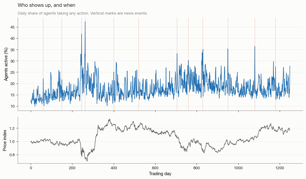
Participation against the price path that produced it. Activity is not uniform: it spikes when the market breaks and stays elevated through the drawdown.
On an average day 18 percent of agents do something, and participation is 1.78 times higher on news days. What matters more than the average is how unevenly it is spread across agents: the median agent acts on 15 days a year, the mean is 45, and the busiest tenth account for 32 percent of all activity. A small minority doing most of the trading is a fact that also holds in real markets.
Attention clusters
Episode 1’s auction alone, with independent agents, produced no volatility clustering. This was expected, since independent zero-intelligence agents have no correlated behaviour by construction. Attention supplies that correlation: a news event makes many agents look at once, their orders move the price, and a large move is itself a trigger that pulls in more agents the next day.
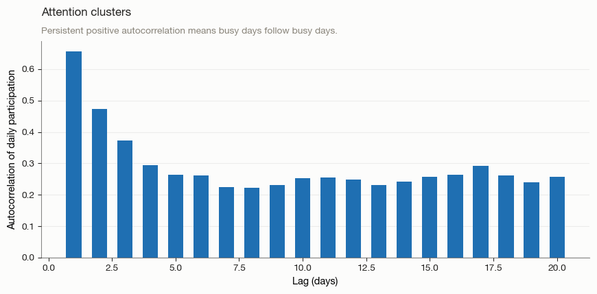
Autocorrelation of daily participation. Busy days follow busy days, still visible twenty days out.
Participation autocorrelation is +0.66 at 1 day and still +0.27 at 5 days. Clustered attention is what makes clustered volatility possible once orders and prices are included. Whether it actually delivers the stylized facts will be discussed in Episode 5, but Episode 1 had no mechanism that could have produced them at all.
What Comes Next
Everything above decides who acts, not what they think. Only the review reason to trade will need a model to be called, and its output has to become two numbers: a valuation and a conviction which will be fed into our demand function. The implementation details will be discussed in the next episode.
Common Questions
Why not let the AI agents decide whether to act?
This would create more opportunities for the model to be inconsistent. Attention is a mechanical, well-studied process, and implementing it outside the language model lets us understand and debug the system better.
Is this how real markets behave?
At this stage, we are not reproducing real market conditions yet. However, the attention mechanism introduced here is consistent with empirical facts and research.
References
- Milgrom & Stokey, “Information, Trade and Common Knowledge”, Journal of Economic Theory (1982): the no-trade theorem — rational agents with common knowledge and no other motive cannot agree to a trade, the reason this article needs a source of trade beyond disagreement.
- Merton, “A Simple Model of Capital Market Equilibrium with Incomplete Information”, Journal of Finance (1987): investors only know a subset of available securities, the basis for the visibility subsample.
- Ma, “Individual Investors’ Dispersion in Beliefs and Stock Returns”, Financial Management (2022): investors looking at the same fundamentals still form different views, the basis for the random per-agent screen weights.
- Masters, “Rebalancing”, Journal of Portfolio Management (2003): the calendar-or-tolerance-band hybrid behind the rebalance rule in section B, and the standard citation for that industry practice.
- Kyle, “Continuous Auctions and Insider Trading”, Econometrica (1985) and Glosten & Milgrom, “Bid, Ask and Transaction Prices in a Specialist Market with Heterogeneously Informed Traders”, Journal of Financial Economics (1985): why informed trading needs uninformed flow to exist alongside it.
- Barber & Odean, “All That Glitters: The Effect of Attention and News on the Buying Behavior of Individual and Institutional Investors” (2008): attention-driven trading, the direct antecedent for the review process.
- Odean, “Volume, Volatility, Price, and Profit When All Traders Are Above Average”, Journal of Finance (1998): overconfidence as a source of excess trading volume.
- Karlsson, Loewenstein & Seppi, “The Ostrich Effect: Selective Attention to Information” (2009): investors check their portfolios less when markets fall, the source of the reduced-attention multiplier.
- Cont & Bouchaud, “Herd Behavior and Aggregate Fluctuations in Financial Markets” (2000): correlated behaviour as a precondition for fat tails and volatility clustering.
Related Cookbooks
Agentic Market Simulator, Part 1: The Engine and the Environment | SR Cookbooks
Part 1 of a 10-part series simulating a stock market traded by language-model agents. Build the call-auction clearing engine and benchmark it against zero-intelligence controls before any model is involved.
Agentic Market Simulator, Part 2: Universe, Information and Leakage | SR Cookbooks
Part 2 of a 10-part series simulating a stock market traded by language-model agents. Move from a synthetic fundamental to real S&P 500 data, measure lookahead bias with a fabricated-financials experiment, and build a re-identification probe to test anonymization.