Agentic Market Simulator, Part 4: Beliefs, Personas and Track Record

Q: Why not ask the model for a price target?

Nothing about a language model's numeric output is calibrated, and a number that looks like a valuation invites everything downstream to treat it as one. Return bins give the model a scale it can reason about, the probabilities give its uncertainty for free, and the step from those to a price is a published formula that can be argued with and changed in one place.

Q: Would sampling not give more varied agents?

It would give varied agents for no reason. Two agents reading the same data with the same history would disagree because of a random draw that is not traceable to anything. In this design, agents differ through their persona, their portfolio, their track record and when they happen to look, all circumstances the simulator can inspect.

Q: Does the model know which company it is looking at?

Not in these experiments: the companies are synthetic, and every input is shown relative to peers, with a pseudonym instead of a name. On real companies, this kind of normalization brings a model's ability to identify a company from its figures close to zero, although not to zero for every model.

This article covers one component of a larger system and makes no claim to replicate a real exchange. Realism will arrive cumulatively across the series: each part is held to its own scope only.

Nothing in this series should be understood as forecasts for prices or investment advice.

In this episode, we discuss how simulated agents form beliefs, and how those beliefs map into buy and sell orders which then shape a simulated market. We present some of the experiments that should be conducted to calibrate and verify the design. While the list is not exhaustive, we aim to give an overview of the areas that matter most, as well as providing solid grounds for understanding how Language Models can be used to form beliefs about assets in the market.

Context Refresh

In Episode 3, we discussed the participation layer, which decides each day which agent looks at which company, and for which reason. When an agent reviews a company, it has to form a view, and that view has to reach the market in the form the Episode 1 auction understands: a demand curve. Writing $i$ for an agent and $p$ for a price, the demand curve is:

q_i^{*}(p) \;=\; \frac{M_i}{1 + \exp\!\big(-k_i \,\log(v_i / p)\big)}

$q_i^{*}(p)$ : the number of shares agent $i$ wants to hold if the price is $p$ .
$M_i$ : the agent’s position limit, the most shares it may hold.
$v_i$ : the agent’s valuation. At $p = v_i$ the agent wants exactly half its limit; below it wants more, above it wants less.
$k_i$ : the agent’s conviction, how sharply its wanted holding changes as the price moves away from $v_i$ .

Every belief an agent forms therefore has to end up as two numbers: the valuation and the conviction. This episode details exactly how $v_i$ and $k_i$ are computed.

Belief Formation

Ordinal Views

A direct and simple approach would be to ask the model for a fair value in dollars. A language model will produce one if asked, but nothing about its numeric output is calibrated: the number looks like a valuation without carrying the information a valuation should. Instead, we ask the model for an ordinal judgement on a fixed rubric: its expected return on the share price over the next quarter, as one of seven labelled bins presented below.

Bin	Shown to the model	Midpoint $m_b$
A	−15% or worse	−20%
B	−15% to −5%	−10%
C	−5% to −1%	−3%
D	−1% to +1%	0%
E	+1% to +5%	+3%
F	+5% to +15%	+10%
G	+15% or better	+20%

The rubric the model answers on. The two open-ended bins take a midpoint five points past their edge.

The question and its horizon are an illustrative choice for this episode. In practice, agents may be asked different questions, over different horizons, and this mix is part of the overall calibration process. The one we use in this episode is there to demonstrate the mechanism and the rubric approach; it should not be taken as one golden rule. The view is about the share price alone. What the agent already holds is shown as context, but the prompt asks for a view that does not depend on it, and the engine will turn that view into a position.

Reasoning & Answer

Each review is one model call which has two steps. In the first step, the model writes one or two sentences on what drives its view, which makes every belief auditable. In the second step, we re-inject the prompt and the previously generated reasoning back with ANSWER: appended at the end. Instead of letting the model generate the rest of the sequence, we extract the next-token probability vector.

The two steps of one review.

It is important to note that the probabilities are not something the model writes explicitly. They are read from the model’s own next-token distribution at the position where the answer letter goes: the probability it assigns to “A”, to “B”, and so on to “G”. A model asked to state its confidence in words tends to be overconfident (Xiong et al., 2024), whereas the token distribution measures its uncertainty directly, and on multiple-choice questions it is reasonably well calibrated for capable models (Kadavath et al., 2022). This is what lets the same call give both a view and a degree of confidence in it.

From probabilities to valuation and conviction

The mapping from the model’s distribution to the two numbers of the demand curve takes three steps, the same for every persona. A small model is often overconfident, putting over 90 percent on a single bin for a quarterly return, so the distribution is first softened with a temperature, the standard way to calibrate an overconfident network (Guo et al., 2017):

\tilde p_b = \frac{p_b^{1/T}}{\sum_{c=A}^{G} p_c^{1/T}}

\hat r_i = \sum_{b=A}^{G} \tilde p_b\, m_b, \qquad \hat\sigma_i = \sqrt{\sum_{b=A}^{G} \tilde p_b\,(m_b - \hat r_i)^2 + \sigma_{\min}^2}

v_i = P_{j,t-1}\,(1 + \hat r_i), \qquad k_i = \min\!\Big(k_{\max},\, \max\!\big(k_{\min},\, \gamma / \hat\sigma_i^{2}\big)\Big)

$b$ : a bin, one of the seven letters A to G.
$p_b$ : the probability the model puts on letter $b$ as its next token, rescaled so the seven sum to one.
$T = 1.5$ : the temperature. Above 1, it moves some probability from the bin the model favours most to its neighbours; bins at zero stay at zero.
$\tilde p_b$ : the softened probability of bin $b$ , which the next formulas use.
$m_b$ : the midpoint of bin $b$ , from the table above.
$\hat r_i$ : the agent’s expected return over the next quarter, the probability-weighted average of the midpoints.
$\hat\sigma_i$ : the agent’s uncertainty, the spread of the softened distribution around $\hat r_i$ .
$\sigma_{\min} = 3\%$ : a floor on the uncertainty, equal to the gap between neighbouring central midpoints, since the bins cannot express certainty finer than that.
$P_{j,t-1}$ : the last closing price of company $j$ , the one under review, before day $t$ .
$v_i$ : the valuation, the last close moved by the expected return.
$k_i$ : the conviction, larger when the model is surer.
$\gamma = 0.02$ : one risk tolerance shared by every persona; $k_{\min} = 0.5$ and $k_{\max} = 8$ bound the conviction. These three and the temperature are placeholders until Episode 6 calibrates them.

The conviction shrinks with the square of the uncertainty: an agent sure of its view trades a lot on it, and an agent hesitating between several bins trades little. For example, a model split between B and F trades far less than one sure of F. This is the mean-variance rule of Markowitz (1952), in which the size of a position grows with the expected return and shrinks with its variance.

Every design choice in this component lies in the bin midpoints, the temperature and the constants above. They are the same for every persona, and may be adapted in later episodes to calibrate the simulator.

One example review process. The bars and numbers are those of the example below.

Example

A value investor reviews a company whose price has just crashed, 20 percent in a week and 25 percent in three months, and which now looks cheap against its peers. The model replies:

“The sharp 25% decline over three months suggests a significant market overreaction to temporary concerns, creating a compelling value opportunity given the company’s cheap valuation metrics relative to peers and its average fundamentals. As a systematic value investor, I expect the price to mean-revert toward its intrinsic value over the next three months.”

The figure below shows the model’s probabilities over the seven bins and how these map to a valuation and a conviction:

From probabilities to valuation and conviction. Each column is one bin of the rubric.

Next, we show what those two numbers mean for trading. Assuming the agent currently holds half its limit, the demand curve says how much it would like to hold at each price the auction could clear at:

From valuation and conviction to orders. In the auction, this curve is submitted as a ladder of limit orders, exactly as in Episode 1.

What the Agent Sees

The prompt below is an example and should not be interpreted as optimal in any sense. It is the one behind the example above and contains the following: the persona and the instructions, then the agent’s portfolio and track record, then the company and why the agent is looking at it today. The company is anonymized following the Episode 2 learnings, with a pseudonym instead of a name and its fundamentals shown against the companies the agent follows.

You are a systematic value investor. You buy companies that look cheap relative to their fundamentals, because you expect the market to correct mispricings over time, and you avoid companies that look expensive. You judge a share by its price relative to its fundamentals, not by its recent price trend.

You will be shown your portfolio, your track record, and one company. Give your
view of the company's share price return over the next 3 months (63
trading days), as one of these bins:

A = -15% or worse
B = -15% to -5%
C = -5% to -1%
D = -1% to +1%
E = +1% to +5%
F = +5% to +15%
G = +15% or better

Your view is about the share price itself. How much of it you then hold is decided
separately, so do not let your current position change the view.

First, in one or two short sentences, say what is driving your view. Then finish
your reply on its own line with exactly:
ANSWER: <letter>

Your portfolio: total value 57,760, cash 40,000.
- C42: 60 shares at 100.00, weight 10.4%
- C21: 150 shares at 41.00, weight 10.6%
- C34: 60 shares at 93.50, weight 9.7%

Your track record: you have no graded calls yet.

Company C42, share price 100.00
Fundamentals, compared with the other companies you follow:
- Price versus earnings: cheaper than 69% of the companies you follow (cheap)
- Price versus sales: cheaper than 69% of the companies you follow (cheap)
- Revenue growth: about average among the companies you follow
- Operating margin: about average among the companies you follow
- Debt: about average among the companies you follow
Price change: 1 week -20.0%, 1 month -24.0%, 3 months -25.0%, 12 months -15.0%.
It trades 30% below its 12-month high. Volatility: more volatile than 97% of the companies you follow (very volatile), 60% a year.
Market over the last 3 months: +0.0%.
News today: none.

You have not reviewed this company before.
You are looking at it today because its price moved sharply this week.

Tuning this prompt is part of improving the quality of the whole system, and it should be judged on how the agents behave. For example, three aspects moved the quality significantly in our tests:

Ranks in words. Fundamentals are shown as the share of followed companies they beat (“cheaper than 69%”) instead of as signed numbers.
No purchase price. Holdings are listed at today’s price, not at what the agent paid, which keeps the view independent of the position.
The price level in words. “It trades 30% below its 12-month high” instead of a simple signed drawdown number.

The persona is at the start of the prompt. It is a short description of an investment style, written once per persona. The five personas that form views are listed in the next section; the passive indexer from Episode 3 never forms a view and is not prompted.

Do Personas Behave as Described?

This is one of the biggest questions to ask when it comes to personas. A persona prompt is only useful if the views it produces differ in the way its description implies. We test that directly by moving one input at a time and watching how each persona’s expected return responds.

Experiment design

Each persona reviews a company whose inputs are all ordinary except one, which is set to a low, a middle and a high level: valuation from two standard deviations expensive to two cheap, 3-month momentum from −30 to +30 percent, the distance below the 12-month high from 0 to 50 percent, and annualized volatility from 12 to 75 percent. We measure the response of a persona to an input as the change in its expected return from one end of that range to the other, in percentage points.

Before running anything, here are some realistic expectations one could have for each persona:

Persona	Described as	Implied response
Value quant	judges price against fundamentals, not by its trend	up with cheapness
Momentum chaser	follows established trends, ignores moves of a few percent	up with momentum, down with drawdown
Risk averse fund	dislikes volatility and deep falls	down with volatility and with drawdown
Retail trader	follows recent performance and headlines	up with momentum
Panic seller	calm by default, frightened by falls	up with momentum, down with drawdown and volatility

Language models can be sensitive to wording, so every response is measured under two wordings of the instructions and two wordings of each persona, and averaged over ten different companies. In total this is 2,400 cases: 5 personas, 4 inputs, 3 levels each, 4 wordings and 10 companies.

Results

The figure below shows each response as a curve. Each panel moves one input from left to right while everything else stays ordinary. The vertical axis is how much the persona’s expected return for the next quarter changes, compared with the same company at its ordinary level, which is why every line passes through zero at the middle point. A line that rises to the right means the persona grows more optimistic as the input increases; the shaded band around it shows how much the result moves across the four wordings.

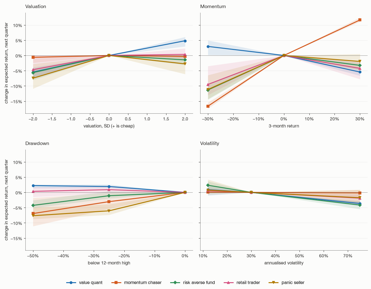
Four panels, one per input, showing how each persona's expected return for the next quarter changes against the same company at its ordinary level. On momentum, the momentum chaser rises from about minus 17 points at a 30 percent fall to plus 12 points at a 30 percent rise, while the other personas are lower for large moves in either direction. On valuation, an expensive company lowers most views by about 5 to 7 points and a cheap one raises only the value quant's, by about 5 points. On drawdown, the panic seller falls by about 7.5 points at 50 percent below the high. On volatility, views fall slightly as volatility rises.

How each persona’s view responds to one input at a time: mean over ten companies, with shaded bands spanning the four wordings.

Overall, the personas are directionally correct: almost every response the descriptions imply shows up with the right sign under every wording, and the size of each response can be read off the curves:

Momentum chaser. Its expected return moves by about 28 points between a 30 percent fall and a 30 percent rise, and it ignores valuation.
Value quant. Moves by about 10 points from an expensive company to a cheap one, and is the only persona that cheapness makes more optimistic.
Panic seller. Loses about 8 points of expected return as the price falls 50 percent below its high.
Risk averse fund. Loses about 6 points as volatility rises from 12 to 75 percent, and about 4 points on a deep fall.
Retail trader. Follows momentum by about 5 points, and is also the one that moves most with the wording, most likely because retail traders are a very generic and heterogeneous category.

We note that two patterns are shared by most personas: an expensive company lowers their view, and a large move in either direction makes the personas that do not chase trends more cautious.

Further tuning of the persona descriptions and the prompt can improve these response curves. The point of this experiment is the methodology: whenever a persona, the prompt or the model changes, sensitivity tests of this kind should be run again before the agents are trusted in a simulated market.

Model choice

We have seen that the choice of model changes these results, because models differ in how well they follow a persona and in how much their answers move with wording. Small models are key to scalability, since a simulation of thousands of agents makes a very large number of calls, but they also come with limitations, and choosing the model is an important part of the design. For this episode we use Qwen3.5-9B. It is a choice for illustration, not necessarily the one a production system would make.

From Scenario to Price

The response curves above isolate one input at a time. Real situations will move several at once, so we now give all five personas the same company in four combined scenarios, and follow each belief all the way to the price it produces.

Four scenarios

Scenario	Valuation	3 months	12 months	Below high	Volatility
Cheap after a long fall	cheaper than 90%	−20%	−30%	35%	40%
Expensive and rising	more expensive than 90%	+20%	+45%	0%	30%
A sudden crash	cheaper than 69%	−25%	−15%	30%	60%
Steady and unremarkable	average	+2%	+6%	3%	22%

The next figure shows, for each scenario, the probability each persona puts on each bin: one row per persona, one column per bin from A (a fall of 15 percent or more) to G (a rise of 15 percent or more). The darker the cell, the more probability the model puts there.

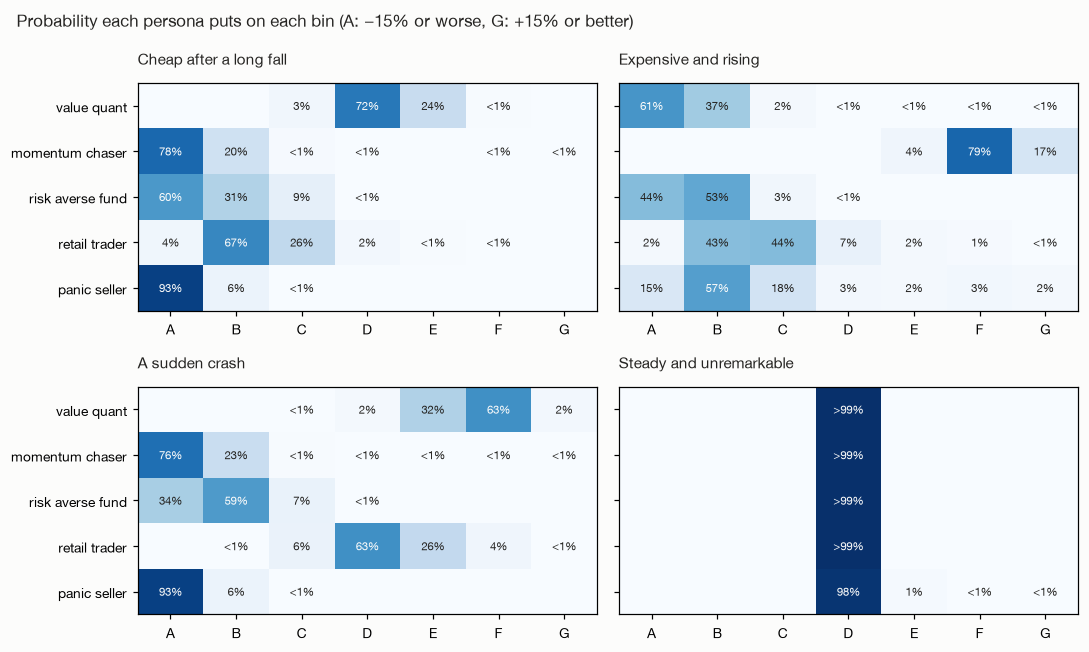
Four heatmaps of the probability each persona puts on each bin. Cheap after a long fall: the value quant puts 72 percent on D while the momentum chaser and panic seller put 78 and 93 percent on A. Expensive and rising: the momentum chaser puts 79 percent on F while the value quant and risk averse fund sit on A and B. A sudden crash: the value quant puts 63 percent on F and the retail trader 63 percent on D and 26 percent on E, while the panic seller puts 93 percent on A. Steady and unremarkable: all five personas put almost all their probability on D.

The probability each persona puts on each bin, for the same company in four scenarios. “<1%” marks a probability between 0.1% and 1%; blank cells are below 0.1%.

In the crash, the value quant sees an opportunity (63 percent on F) and the retail trader leans the same way, while the momentum chaser and the panic seller see a trend that will continue (76 and 93 percent on A). After a slower fall the value quant is more hesitant, mostly on D, and in a rising, expensive market the roles reverse. Here are 2 examples of the reasoning given by agents during the crash:

“This stock has plummeted 25% in just three months and trades significantly below its recent high, triggering my fear that the downward momentum will continue rather than reverse soon.” (panic seller)

“The stock has already dropped 25% over the last three months and is trading 30% below its 12-month high, suggesting the recent sharp decline may be an overreaction to bad news that has already been priced in.” (retail trader)

In the steady scenario, by contrast, all five personas put almost all their probability on D: an unremarkable company gives them no reason to expect anything. This over-confidence is not necessarily the most realistic pattern for steady assets, and can be tuned through the smoothing parameter. This will be part of the calibration process in later episodes.

Demand curves

Each of these distributions becomes a valuation, a conviction and a demand curve, as in the example above. In the next figure, the horizontal axis is the price at which the auction could clear, with the previous close at 100, and the vertical axis is the number of shares the agent wants to hold at that price, as a share of its position limit. Every agent starts holding half its limit, marked by the dotted line. Where a curve is above the dotted line, the agent buys at that price; where it is below, the agent sells. The point where a curve crosses the dotted line is that agent’s valuation, and the steeper the curve, the higher its conviction.

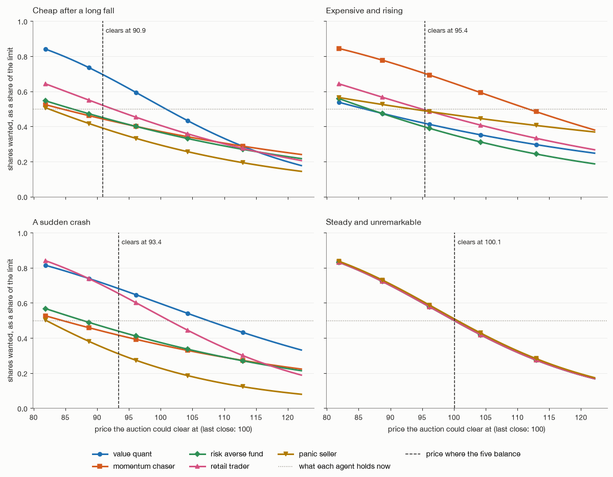
Each persona’s demand curve in each scenario. The dashed line is the price at which the five agents’ buying and selling balance.

Sample Auction with 5 Agents

To see a price form, we run a small experiment for illustration: one agent of each persona, each with the same position limit and starting with holdings equal to half of the limit. In that setup, any trade comes from disagreement. The clearing price is the one at which supply meets demand: the shares the buyers want to add equal the shares the sellers want to shed; in other words, their net demand is zero. This is the price Episode 1’s call auction finds when it maximizes the volume that changes hands (see Episode 1 for full details about the auction system); here we solve for it directly from the five demand curves, within the ±20 percent daily limit.

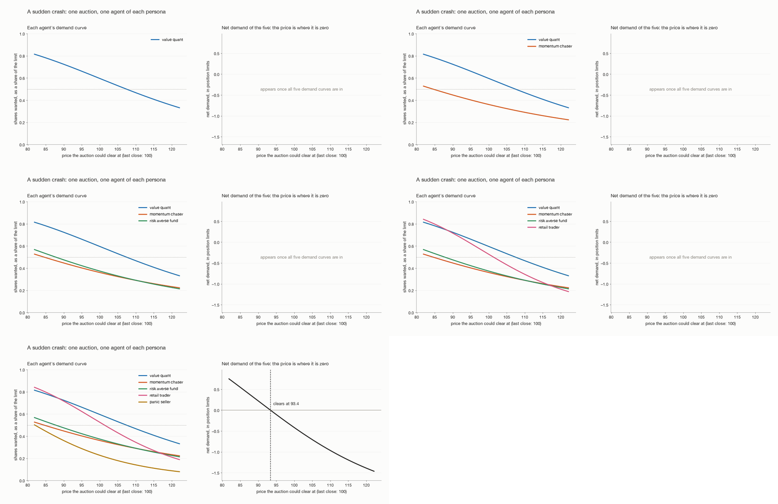
Animation of the sudden crash scenario. Five demand curves appear one at a time, one per persona: the value quant's and the retail trader's sit far to the right of the others. Once all five are shown, a second panel draws their combined net demand, which crosses zero at a price of 93.4.

The crash scenario, one persona at a time. The price is where the five curves’ net demand crosses zero.

Scenario	Clears at	Main buyers	Main sellers
Cheap after a long fall	90.9	value quant (+20%), retail (+2%)	panic seller (−11%), momentum chaser (−6%)
Expensive and rising	95.4	momentum chaser (+20%)	risk averse fund (−10%), value quant (−8%)
A sudden crash	93.4	value quant (+18%), retail trader (+15%)	panic seller (−19%), momentum chaser (−8%)
Steady and unremarkable	100.1	none	none

Last close 100. Trades are shown as a share of each agent’s position limit, at the clearing price.

In every scenario the price lands where buyers and sellers with opposite readings of the same company balance. After a long fall, the sellers outweigh the buyers and the price drops another 9 percent, with the value quant absorbing most of what is sold. In the crash, the value quant and the retail trader are the counterparties to the panic, and the price falls only 7 percent. The steady company does not move, because the five agents agree.

The roles roughly match known investor behavior. Buying recent winners is the momentum effect documented by Jegadeesh and Titman (1993); buying after large falls and selling after large rises is the contrarian trade behind De Bondt and Thaler’s (1985) evidence of overreaction; and individual investors in particular trade as contrarians, buying stocks that have just declined (Kaniel, Saar and Titman, 2008). Above all, the agents disagree, which Milgrom and Stokey (1982) showed is what any trade requires: same data, same portfolio, same model, and five different positions.

Track Record

Two agents with the same persona reading the same data should not stay interchangeable once their individual track records have gone differently. This is the mechanism Brock and Hommes (1998) placed at the centre of their heterogeneous-agent model, where traders weigh strategies by their past performance; here the history is given to the model as context, and the model decides what to make of it.

How the record enters the prompt

Every view an agent forms is graded a quarter later, the horizon it was a view about, against what the share price did and what the market did over the same window. The graded calls, up to the last 50, appear in the agent’s prompt under a one-line summary. An agent whose last six calls all went the wrong way sees:

Your track record: 6 graded calls: inside your range on 0, direction right on 0 of 6, average outcome -0.2% versus your bin's midpoint.
- day 7: C11, you said F (+5% to +15%); it moved -9.4% (market +2.1%), below your range
- day 16: C12, you said B (-15% to -5%); it moved +8.7% (market +1.0%), above your range
- day 25: C13, you said E (+1% to +5%); it moved -3.2% (market +1.5%), below your range
- day 34: C14, you said C (-5% to -1%); it moved +2.6% (market +0.8%), above your range
- day 43: C15, you said F (+5% to +15%); it moved -11.8% (market +2.4%), below your range
- day 52: C16, you said B (-15% to -5%); it moved +12.1% (market -0.5%), above your range

Experiment design

Each persona reviews the same company in 14 situations (the four scenarios above and ten ordinary companies), three times, each time with a different track record:

No record. The agent has never made a call before.
A good record. Six past calls on other companies, every one of which was right: when the agent expected the price to go up, it went up, and when it expected the price to go down, it went down.
A bad record. The same six calls with every outcome reversed, so every one of them was wrong. This is the record shown above.

In both records, three of the six past calls expected the price to go up and three expected it to go down. A record therefore tells the agent how good its past calls were, without hinting at whether prices in general have been rising or falling. Everything else in the prompt stays the same, so any difference in the view comes from the record alone. Across the five personas, that is 210 cases.

What the record changes

The next figure compares two agents of the same persona looking at the same company, one with the good record and one with the bad one. The left panel shows how far apart their expected returns are on average, the right panel how often they pick a different bin.

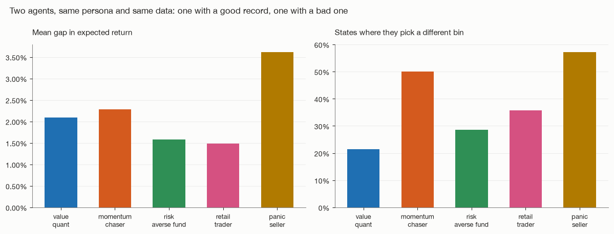
Two bar charts by persona comparing an agent with a good record and one with a bad record, on the same data. Left: the mean gap in expected return, 3.6 points for the panic seller and 1.5 to 2.3 points for the others. Right: the share of states where the two pick a different bin, 57 percent for the panic seller, 50 percent for the momentum chaser, 36 percent for the retail trader, 29 percent for the risk averse fund and 21 percent for the value quant.

Two agents of the same persona on the same data, one with a good record and one with a bad one, over 14 states.

Persona	Different bin	Mean gap in expected return
Panic seller	57%	3.6 pts
Momentum chaser	50%	2.3 pts
Retail trader	36%	1.5 pts
Risk averse fund	29%	1.6 pts
Value quant	21%	2.1 pts

For every persona, the record alone changes the bin the agent picks in 21 to 57 percent of states. On individual states the effect can be large. The value quant looking at the company after a long fall is close to neutral with no record (+0.8 percent), but turns to −6.8 percent with a good record and −17.4 percent with a bad one. The next figure shows its three demand curves, read the same way as before:

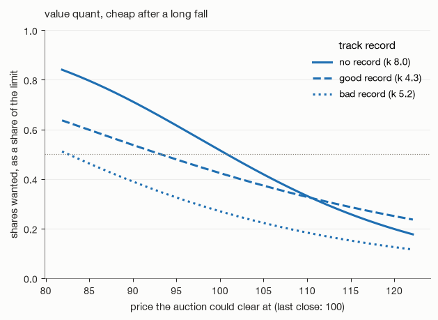
Three demand curves of the value quant for the company that is cheap after a long fall. With no track record the curve crosses one half at about 101; with a good record at about 93, and with a bad record at about 83, so with either record the agent becomes a seller at the current price of 100.

The same value quant, the same company: close to neutral with no record, a seller with either record.

How a record changes the view does not follow a simple rule. Only the panic seller reacts the way one might expect: after a run of wrong calls it becomes more pessimistic, and its average expected return across the 14 situations falls from −4.3 percent with no record to −7.0 percent. For the other personas, simply having a record often changes the view as much as whether that record is good or bad. What matters for a simulator is that the record makes a difference at all: once their histories differ, agents of the same persona stop being copies of each other.

A Small Market Over a Year

A single auction shows how a price forms from one set of views. A market repeats it every day, and the price an auction sets today becomes the momentum, drawdown and valuation an agent reads tomorrow. To see that loop close, we run every layer of the series together for one simulated year, at a size small enough to run on a laptop.

Setup

Three synthetic companies, one positive, one neutral and one negative. They share one ordinary year of history before day 0, in which the price rose 6 percent with realistic daily noise. From day 0, the positive company reports four quarters of earnings up 8 percent with growth and margins rising, the negative company the reverse, and the neutral company results in line. Results dates are staggered by a few days between companies, as in a real reporting season.
News arrives at random times. A calendar adds company news on random days: four good items and one bad for the positive company, one good and four bad for the negative company, and two of each for the neutral one. Four market-wide events, two good and two bad, reach every company. Each item is a flat, factual line such as “The company announced the loss of a major customer”.
Agents see everything filed so far. Each review lists the quarterly results published to date, as Episode 2 specifies that agents see every report filed. Valuation is measured against the simulated price, so a rally makes a share look dearer. Different analytical capabilities will be introduced in later episodes.
20 agents: 7 retail traders, 4 value quants, 5 momentum chasers, 3 risk averse funds and 1 panic seller, plus one market maker the size of an average agent. Each agent starts holding half its position limit, the holding it wants when its view equals the price, so every trade comes from disagreement or from a need for cash.
Cash eventAn agent adds or withdraws money. Its position limit moves, so it trades without changing its view.
Episode 3’s participation layer decides who acts. Agents review each name at their persona’s own random cadence, more often after results, news, a large move or a deep fall, and only a review calls the model. Cash events at each persona’s published rate scale an agent’s position limits up or down by 20 percent, which its demand curve then trades in the auction. Between reviews, an agent keeps its last valuation and conviction.
A control runs the same market, seed, agents and news calendar, with each persona’s view taken from its response curves above instead of a model call: a fixed rule with the persona’s average reactions and no memory, which cannot read the results or the news.

Over 250 trading days the agents made 458 model calls. Each day’s reviews are sent to the model as one batch, and every price is set by the Episode 1 call auction, one per company per day.

How Prices Moved

The animation below draws the year day by day. Each panel is one company’s own share price, set every day by its auction: in black when the agents’ views come from the language model, in grey in the control. Solid vertical lines mark the quarterly results, labelled with what they said; triangles mark company news (green for good, red for bad); dotted lines mark market-wide news, with its sign at the foot of each panel. All three panels share one vertical scale, so the size of each move can be compared directly, and the animation pauses on the full year at the end.

Animation of one simulated year, drawn day by day, in three stacked panels, one per company, on one shared price scale. Each shows the company's price with the language-model agents and in the rule-based control, with quarterly results, company news and market news marked as they arrive. The positive company's price rises in steps after good results and good news and ends at 108.8. The negative company's price falls after each bad result and bad news item, from 100 to 50.7. The neutral company stays close to 100 and ends at 102.7. The control prices stay within 8 percent of 100. The animation pauses on the full year at the end.

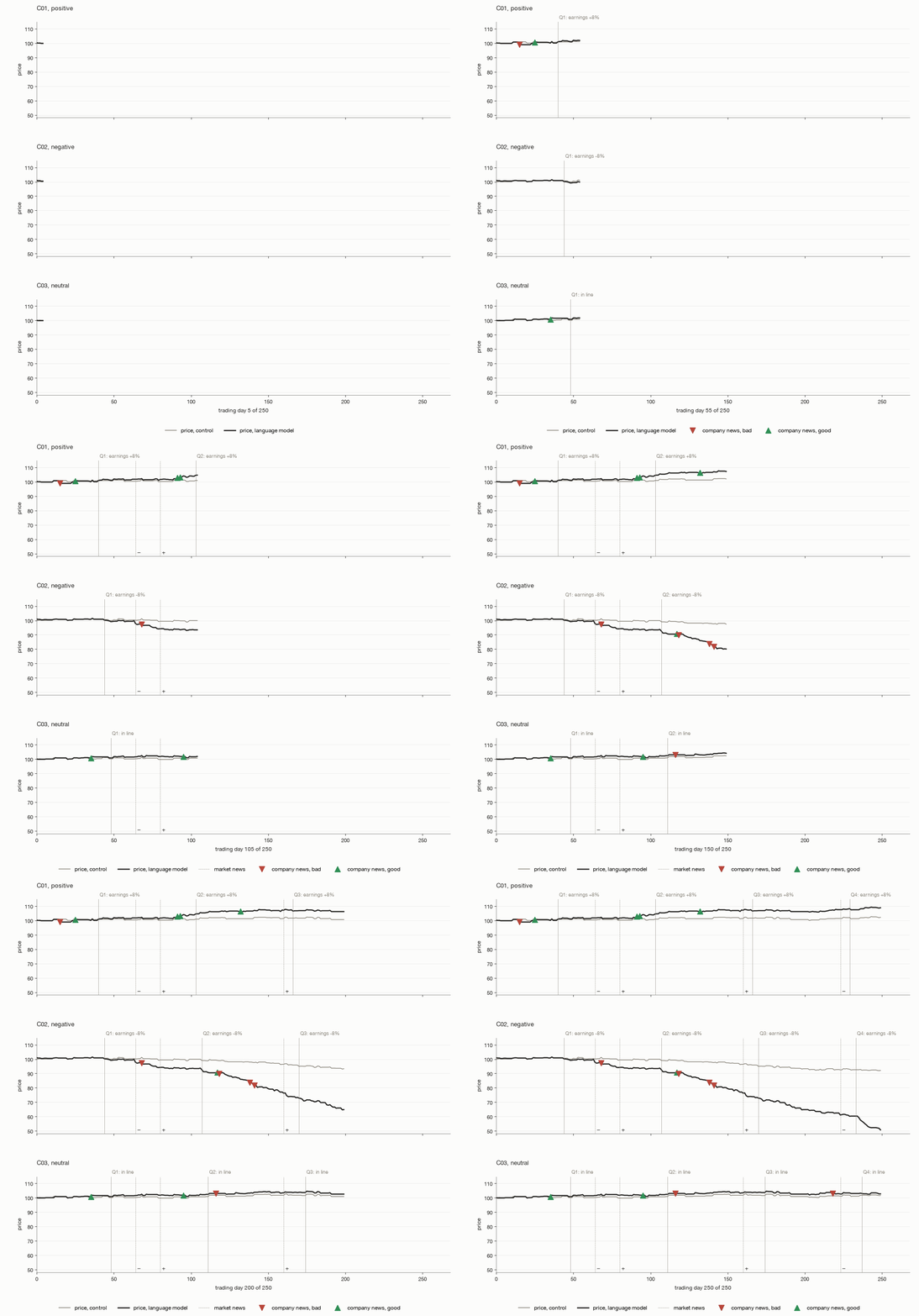
One simulated year for three companies, with every result and news item appearing on the day it reaches the agents.

Company	Earnings over the year	Price, model	Price, control	After each result (model)
Positive	+36%	108.8	102.2	+2.0% +2.1% −0.1% +0.9%
Neutral	0%	102.7	101.6	+0.6% +0.6% −0.4% +0.0%
Negative	−28%	50.7	92.1	−1.0% −3.1% −4.2% −13.4%

Prices at the end of the year, from a start of 100. “After each result” is the change from the close before a filing to ten days after it.

The first thing to notice is that the prices move in the direction of the information, and in the right order: the positive company ends 9 percent up, the neutral company ends close to where it started, and the negative company falls after every bad result. The control, whose rule cannot read the results or the news, barely moves on any of them. Company news moves prices in its own direction too, in smaller steps: the loss of a major customer takes the negative company down 5.8 percent in the following week, and a contract extension lifts the positive company 1.8 percent.

In the control, a fixed rule reacts to a few numbers, such as how cheap the company looks or how far its price has moved, and reacts the same way every time. With the language model, the agents also read the results and the news as written text, and each forms its own view from them. That is the main benefit of a language model here: inputs can be given in natural language instead of being reduced to a few predefined parameters, and the agents react to them in more varied ways, shaped by their persona and their own history. The gap between the black and grey lines shows that benefit.

The second thing to notice is that the response is asymmetric. Good news is priced gradually, about 1 to 2 percent per result: over the year, the positive company’s earnings rise about 36 percent and its price 9 percent. Bad news is priced strongly: the negative company’s earnings fall about 28 percent and its price 49 percent. In the days after a result or a news item, the agents’ views average +3.8 percent on the positive company and −12.9 percent on the negative one. Real markets show a milder version of the first effect, with prices that under-react to earnings news and keep drifting in its direction for weeks afterwards (Bernard and Thomas, 1989), and traders who are reluctant to bid a stock above its 52-week high (George and Hwang, 2004). Here the gap is much larger, for two reasons.

The first is attention. Episode 3’s drawdown trigger sends extra reviews to a stock that falls far below its 12-month high, and these come from the personas most likely to sell. The negative company receives 169 reviews over the year (110 of them prompted by its fall) against 112 for the positive company, and nothing draws the same extra attention to a stock that keeps rising. The second is the beliefs: the risk averse fund and the panic seller are loss-averse by definition, and the model reacts more strongly to bad news than to good, as the response curves showed.

Both of these can be tuned. A symmetric trigger, such as a stock reaching a new high or rising sharply, would give good news the same extra attention. The persona proportions set how many agents lean toward selling a falling stock, and the persona prompts and the constants of the belief layer set how strongly each reacts. These are calibration choices which we will make against real data in later episodes.

On the positive company, the value quant turns optimistic as each result lands:

“The recent quarterly results show accelerating earnings growth, revenue expansion, and an improved operating margin, confirming that the company’s fundamentals are strengthening while the share price remains cheap relative to peers.” (value quant, day 40, answering F)

The steady part of the rise comes from the momentum chasers, whose views on the positive company average +6.8 percent once its uptrend is established. On the way down, the same trend-following and the panic seller’s fear amplify the move, so the negative company’s price falls further than its earnings.

Who Trades?

The figure below shows each persona’s holding over the year, as a share of its position limit. Every persona starts at one half (dotted line); a line above it means the persona has been buying, below it selling.

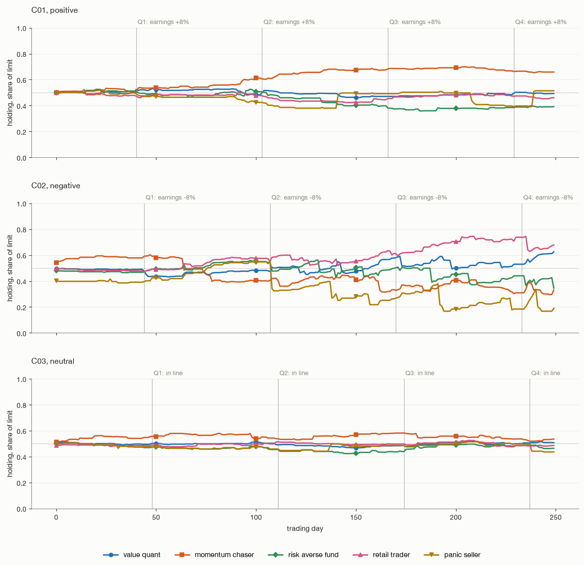
Three stacked panels showing each persona's holding over the year as a share of its position limit, starting at one half. In the negative company, the retail trader rises to about 68 percent and the value quant to about 63 percent, while the momentum chaser, the risk averse fund and the panic seller fall to between 19 and 35 percent. In the positive company the momentum chaser rises to about 66 percent and the risk averse fund falls to about 39 percent. In the neutral company every persona stays close to one half.

Each persona’s holding as a share of its position limit (start: one half).

As the negative company falls, the retail trader and the value quant buy it, ending at 68 and 63 percent of their limits, while the momentum chaser, the risk averse fund and the panic seller sell it down to 33, 35 and 19 percent. The buyers of a falling stock are the same contrarian personas that bought in the single-auction crash. On the positive company, the momentum chaser builds a position as the price rises, ending at 66 percent of its limit. On the neutral company, no persona moves far from where it started.

Agents Drift

The last figure measures how far apart agents of the same persona are: each day, the spread of their valuations relative to the price, averaged over personas and companies.

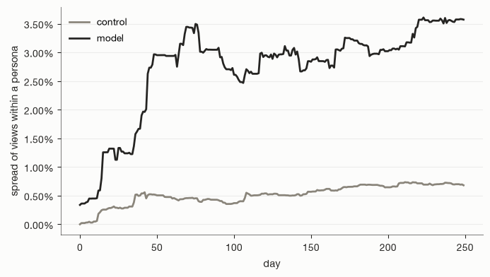
Line chart over the year of the spread of views among agents of the same persona. In the control it stays below 0.7 percent. With the language model it rises after the first results and news and reaches about 3.6 percent by the end of the year.

The spread of views among agents of the same persona: with the language model, and in the control.

In the control, agents of one persona differ only in when they last looked, and the spread of their views stays below 0.7 percent. With the model, each agent carries its own portfolio, previous view and track record into every review, and the spread reaches about 3.6 percent by the end of the year. This also shows the benefit of Language Models compared to static rules to model agents: it creates a more diverse set of views within agents which generates conditions for trade to happen.

How this compares with real markets

Each directional pattern in this market has a documented counterpart in real markets:

In this simulated market	In real markets	Source
Prices move in the direction of quarterly results	Stock prices move in the direction of earnings news	Ball and Brown (1968)
Good results are priced gradually, over several quarters	Prices under-react to earnings news and keep drifting in its direction; near a 52-week high, traders are slow to bid prices up	Bernard and Thomas (1989); George and Hwang (2004)
Bad news moves prices more than good news	Negative earnings surprises can bring disproportionately large price falls, notably for growth stocks	Skinner and Sloan (2002)
Prices keep falling in the weeks after bad company news	Strong price drift after bad news headlines, mainly in smaller stocks	Chan (2003)
The fearful personas react more to losses than to gains	Losses weigh more than gains of the same size	Kahneman and Tversky (1979)
Retail traders and value investors buy the falling stock; trend followers buy the rising one	Individual investors trade as contrarians; trend-following momentum is persistent	Kaniel, Saar and Titman (2008); Jegadeesh and Titman (1993)

The directions match, but the magnitudes are not calibrated: the positive company’s price rises about a quarter as much as its earnings over the year, while the negative company’s price falls further than its earnings. Part of this comes from the size of the market, and part from the design: the strength of each persona’s reaction and the attention a falling price draws are not yet calibrated against real data.

Limits of this small market

Important expected market mechanics hold only directionally in this small simulation. Two important factors which will improve the realism are still missing:

Scale. With 20 agents, the book fails to cross on a fifth to a third of days and the market maker carries a large share of the trading. A much larger number of agents will be needed to create more diverse views and sessions that close almost always.
Calibration. This is the most important one. Adjusting simulation parameters discussed so far will help create a more realistic market. For example, in this very small example, we observe that annualized volatility is 5 to 10 percent, against roughly 20 percent for a real large cap. Its level is set by how often new information arrives and how strongly agents trade on it. The next episodes will calibrate the simulation parameters against real data.

We showed in this episode how the belief layer turns one review into a valuation and a conviction. It is the only part of the simulator that calls a language model. The small market shows the full loop working: information arrives, personas react in their own way, the auction runs, and prices move with it. It also shows what a few agents cannot do. The next episode is about running this for a large population: thousands of agents, hundreds of companies and several years of trading days, and what it costs to keep each agent’s own history in its decisions at that scale.

A note on scale

The experiments in this episode are deliberately small: five personas, a handful of synthetic companies, and a market of 20 agents trading for one simulated year on a laptop. Their purpose is to show how the system works end to end, from one prompt to one price, and how the first market patterns start to arise from it: personas taking opposite sides, prices responding to new information, agents of the same style drifting apart. They are not meant to reproduce a real market. Some properties of real markets, such as realistic volatility, fat tails and volatility clustering, do not appear at this size and with these placeholder parameters. The directions observed here are consistent with documented market behavior; their magnitudes are not yet. In the large-scale version, parts of this design will be adjusted and calibrated against real market data.

Common Questions

Why not ask the model for a price target?

Because nothing about a language model’s numeric output is calibrated. The bins give the model a scale it can reason about; the probabilities give its actual uncertainty.

Would sampling not give more varied agents?

Two agents reading the same data with the same history would disagree because of a random draw, and that disagreement would not be traceable to anything. In this design, agents differ through their persona, their portfolio, their track record and when they happen to look, which are all circumstances the simulator can inspect. An important motivation for developing such a simulator is its auditability.

Does the model know which company it is looking at?

Not in these experiments: the companies are synthetic, and every input is shown relative to peers, with a pseudonym instead of a name. On real companies, Episode 2 showed that this kind of normalization brings a model’s ability to identify a company from its figures close to zero.

References

Markowitz, “Portfolio Selection”, Journal of Finance (1952): mean-variance positioning, the reason conviction scales with one over the variance of the view.
Kadavath et al., “Language Models (Mostly) Know What They Know” (2022): token probabilities on multiple-choice answers as a measure of a model’s confidence.
Xiong et al., “Can LLMs Express Their Uncertainty? An Empirical Evaluation of Confidence Elicitation in LLMs”, ICLR (2024): confidence stated in words tends to be overconfident, the reason the probabilities are read from the token distribution.
De Bondt & Thaler, “Does the Stock Market Overreact?”, Journal of Finance (1985): evidence of overreaction and reversal, the logic of the contrarian trade.
Jegadeesh & Titman, “Returns to Buying Winners and Selling Losers: Implications for Stock Market Efficiency”, Journal of Finance (1993): the momentum effect, the behavior of the momentum chaser.
Guo, Pleiss, Sun & Weinberger, “On Calibration of Modern Neural Networks”, ICML (2017): temperature scaling, the step that softens the model’s bin distribution.
Ball & Brown, “An Empirical Evaluation of Accounting Income Numbers”, Journal of Accounting Research (1968): stock prices move in the direction of earnings news.
Bernard & Thomas, “Post-Earnings-Announcement Drift: Delayed Price Response or Risk Premium?”, Journal of Accounting Research (1989): prices under-react to earnings news and drift in its direction afterwards.
Skinner & Sloan, “Earnings Surprises, Growth Expectations, and Stock Returns or Don’t Let an Earnings Torpedo Sink Your Portfolio”, Review of Accounting Studies (2002): an asymmetrically large price response to negative earnings surprises.
Chan, “Stock Price Reaction to News and No-News: Drift and Reversal after Headlines”, Journal of Financial Economics (2003): strong drift after bad news headlines.
Kahneman & Tversky, “Prospect Theory: An Analysis of Decision under Risk”, Econometrica (1979): loss aversion, the behavior the risk averse fund and the panic seller are defined by.
George & Hwang, “The 52-Week High and Momentum Investing”, Journal of Finance (2004): traders anchor on the 52-week high and under-react to good news near it.
Kaniel, Saar & Titman, “Individual Investor Trading and Stock Returns”, Journal of Finance (2008): individual investors trade as contrarians, the pattern the retail persona shows in the crash.
Brock & Hommes, “Heterogeneous Beliefs and Routes to Chaos in a Simple Asset Pricing Model”, Journal of Economic Dynamics and Control (1998): traders weighing strategies by past performance, the antecedent for the track record.
Milgrom & Stokey, “Information, Trade and Common Knowledge”, Journal of Economic Theory (1982): the no-trade theorem, the reason the simulator needs agents that disagree.

Agentic Market Simulator Part 4: Beliefs, Personas and Track Record

Agentic Market Simulator · Part 4 of 10

TL;DR

Context Refresh

Belief Formation

Ordinal Views

Reasoning & Answer

From probabilities to valuation and conviction

Example

What the Agent Sees

Do Personas Behave as Described?

Experiment design

Results

Model choice

From Scenario to Price

Four scenarios

Demand curves

Sample Auction with 5 Agents

Track Record

How the record enters the prompt

Experiment design

What the record changes

A Small Market Over a Year

Setup

How Prices Moved

Who Trades?

Agents Drift

How this compares with real markets

Limits of this small market

Next

A note on scale

Common Questions

Why not ask the model for a price target?

Would sampling not give more varied agents?

Does the model know which company it is looking at?

References

Related Cookbooks

Agentic Market Simulator, Part 3: Actions, Personas and Track Record

Agentic Market Simulator, Part 2: Universe, Information and Leakage

Agentic Market Simulator, Part 1: The Engine and the Environment